Dynamical systems' based neural networks

Davide Murari

davide.murari@ntnu.no

Theoretical and computational aspects of dynamical systems

HB60

What are neural networks

They are compositions of parametric functions

\( \mathcal{N}(x) = f_{\theta_k}\circ ... \circ f_{\theta_1}(x)\)

ResNets

\(\Sigma(z) = [\sigma(z_1),...,\sigma(z_n)],\)

\( \sigma:\mathbb{R}\rightarrow\mathbb{R}\)

f_{\theta}(x) = x + B\Sigma(Ax+b),\\ \theta = (A,B,b)

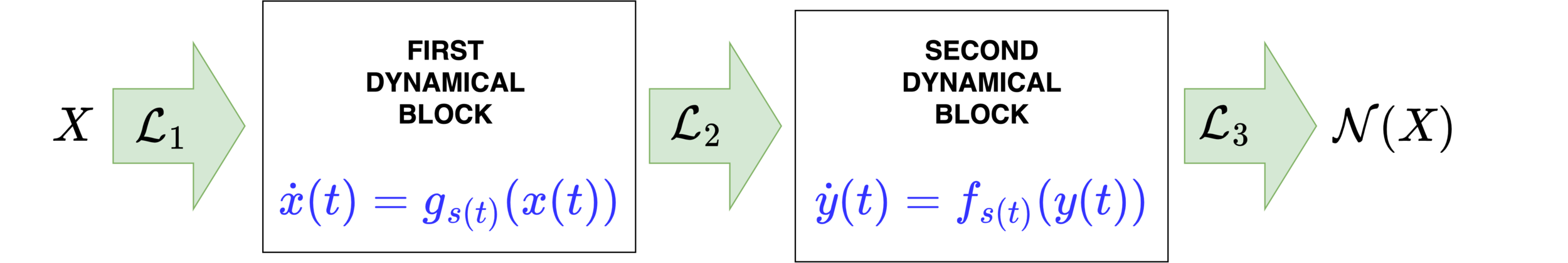
Neural networks motivated by dynamical systems

\mathcal{N}(x) = \Psi_{f_k}^{h_k}\circ ...\circ \Psi_{f_1}^{h_1}(x)

\( \dot{x}(t) = h(x(t),\theta(t))=:h_{s(t)}(x(t)) \)

Where \(f_i(x) = f(x,\theta_i)\)

\theta(t)\equiv \theta_i,\,\,t\in [t_i,t_{i+1})

t_0

t_1

t_2

t_i

t_{i+1}

t_M=T

\cdots

h_i

{

Neural networks motivated by dynamical systems

What if I want a network with a certain property?

GENERAL IDEA

EXAMPLE

Property \(\mathcal{P}\)

\(\mathcal{P}=\)Volume preservation

Family \(\mathcal{F}\) of vector fields that satisfy \(\mathcal{P}\)

\(X_{\theta}(x,v) = \begin{bmatrix} \Sigma(Av+a) \\ \Sigma(Bx+b) \end{bmatrix} \)

\(\mathcal{F}=\{X_{\theta}:\,\,\theta\in\mathcal{A}\}\)

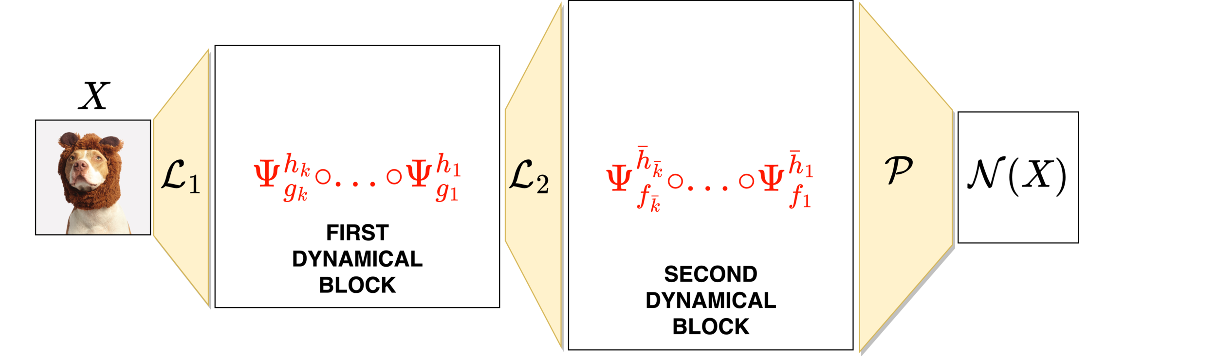
Integrator \(\Psi^h\) that preserves \(\mathcal{P}\)

x_{n+1}=x_n+h\Sigma(Av_n+a)\\ \,\,\,\,v_{n+1}=v_n+h\Sigma(Bx_{n+1}+b)

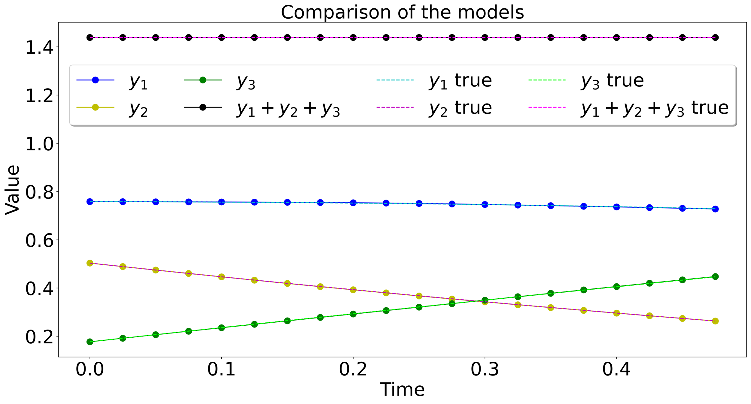
Mass-preserving networks

\dot{y} = \begin{bmatrix} 0 & -y_3y_1^2 & y_2y_3 \\ y_3y_1^2 & 0 & -\sin{y_1} \\ -y_2y_3 & \sin{y_1} & 0\end{bmatrix}\boldsymbol{1}

\dot{x}(t) = \{A_{\theta}(x(t))-A_{\theta}(x(t))^T\}\boldsymbol{1}\\ \mathrm{vec}(A_{\theta}(x)) = \Sigma(Ux+u)

Lipschitz-constrained networks

\(m=1\)

\(m=\frac{1}{2}\)

\(\Sigma(x) = \max\left\{x,\frac{x}{2}\right\}\)

We consider orthogonal weight matrices

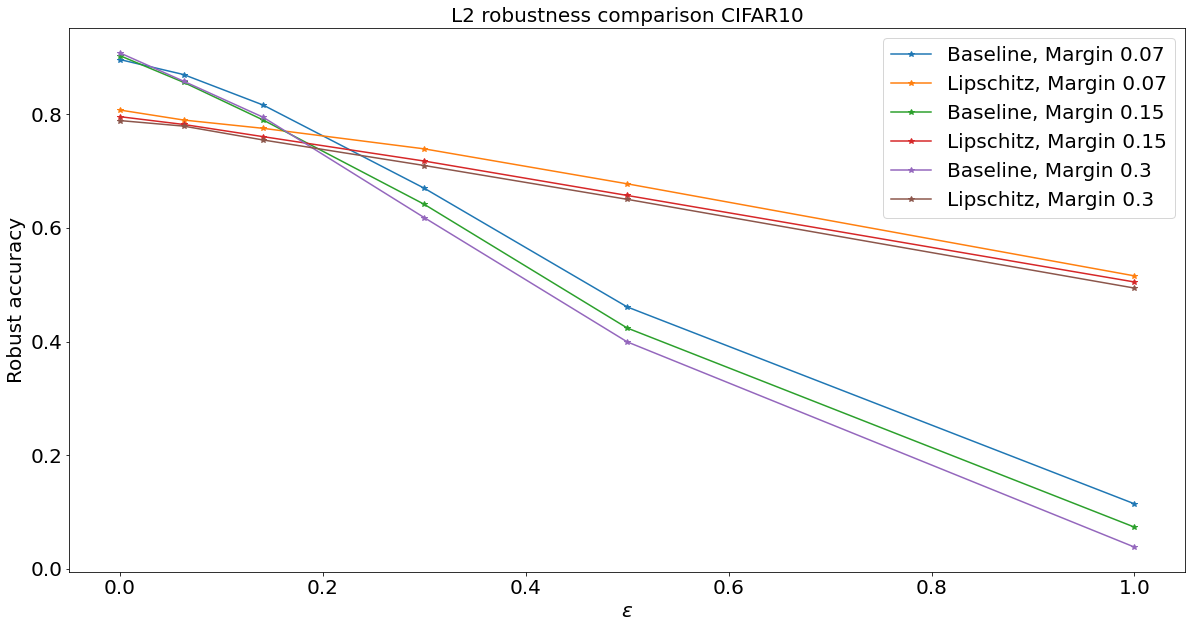
Lipschitz-constrained networks

X_{\theta_i}(x) := - \nabla V_{\theta_i}(x) = -A_i^T\Sigma(A_ix+b_i)

\Psi^{h_C}_{X_{\theta_i}}(x) = x - {h_C}A_i^T\Sigma(A_ix+b_i)

Y_{\theta_i}(x) := \Sigma(W_ix + v_i)

\|\Psi^{h_C}_{X_{\theta_i}}(y) - \Psi^{h_C}_{X_{\theta_i}}(x)\|\leq \sqrt{1-{h_C}+{h_C}^2}\|y-x\|

\Psi^{h_E}_{Y_{\theta_i}}(x) = x + {h_E}\Sigma(W_ix+v_i)

\|\Psi^{h_E}_{Y_{\theta_i}}(y) - \Psi^{h_E}_{Y_{\theta_i}}(x)\|\leq (1+{h_E})\|y-x\|

Lipschitz-constrained networks

\mathcal{N}(x)=\Psi_{X_{\theta_{2k}}}^{h_{2k}} \circ \Psi_{Y_{\theta_{2k-1}}}^{h_{2k-1}} \circ ... \circ \Psi_{X_{\theta_2}}^{h_2} \circ \Psi_{Y_{\theta_{1}}}^{h_1}(x)

We impose :

\|\mathcal{N}(x)-\mathcal{N}(y)\|\leq \|x-y\|

\sqrt{1-{h_C}+{h_C}^2}(1+h_E)\leq 1

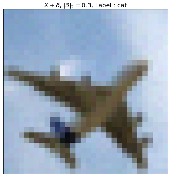
Adversarial examples

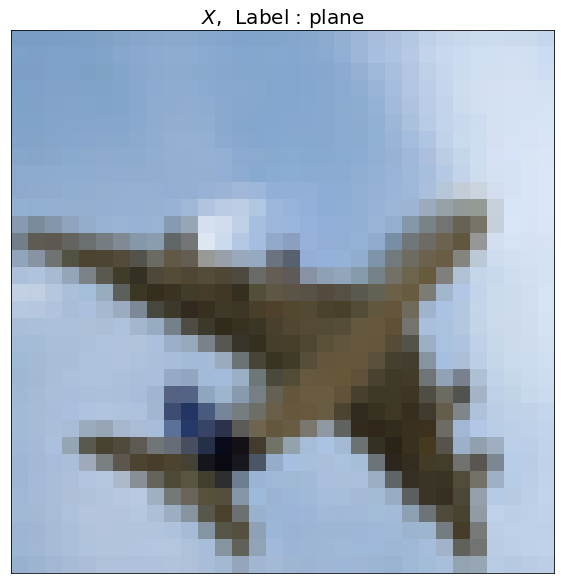
\(X\) ,

Label : Plane

\(X+\delta\),

\(\|\delta\|_2=0.3\) ,

Label : Cat

Thank you for the attention

f_i = \nabla U_i + X_S^i

U_i(x) = \int_0^1 x^Tf_i(tx)dt

x^TX_S^i(x)=0\quad \forall x\in\mathbb{R}^n

Then \(F\) can be approximated with flow maps of gradient and sphere preserving vector fields.

F:\Omega\subset\mathbb{R}^n\rightarrow\mathbb{R}^n\quad \text{continuous, and}

\forall \varepsilon>0\,\,\exist f_1,…,f_k\in\mathcal{C}^1(\mathbb{R}^n,\mathbb{R}^n)\,\,\text{s.t.}

\|F-\Phi_{f_k}^{h_k}\circ … \circ \Phi_{f_1}^{h_1}\|<\varepsilon.

Can we still accurately approximate functions?

\Phi_{f_i}^h = \Phi_{f_i}^{\alpha_M h} \circ ... \circ \Phi_{f_i}^{\alpha_1 h}

\sum_{i=1}^M \alpha_i = 1

f = \nabla U + X_S \\ \implies \Phi_f^h = \Phi_{\nabla U}^{h/2} \circ \Phi_{X_S}^h \circ \Phi_{\nabla U}^{h/2} + \mathcal{O}(h^3)