A numerical analysis perspective on neural networks
Davide Murari
davide.murari@ntnu.no

In collaboration with : Elena Celledoni, James Jackaman, Brynjulf Owren, Carola-Bibiane Schönlieb, and Ferdia Sherry
\( \mathcal{N}(x) = f_{\theta_M}\circ ... \circ f_{\theta_1}(x)\)
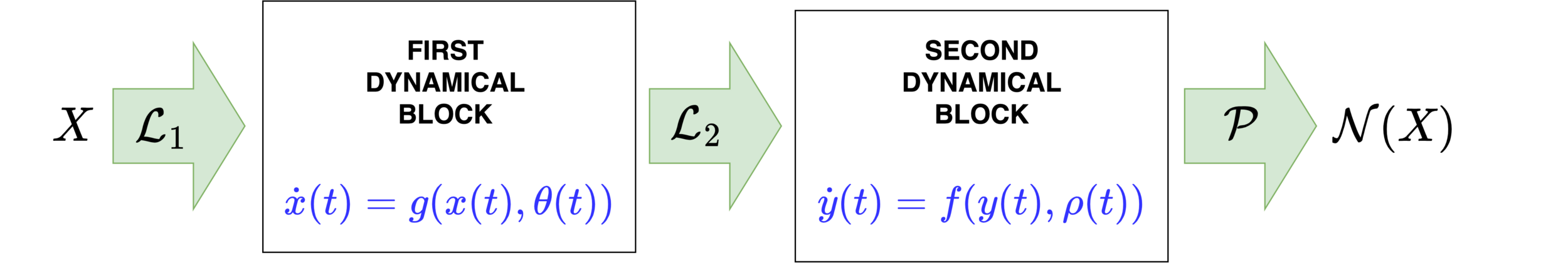
Neural networks motivated by dynamical systems

\( \dot{x}(t) = F(x(t),\theta(t)) \)
Where \(F_i(x) = F(x,\theta(t_i))\)
\( \delta t_i = t_{i}-t_{i-1}\)
\( \mathcal{N}(x) = f_{\theta_M}\circ ... \circ f_{\theta_1}(x)\)
Neural networks motivated by dynamical systems
\( \dot{x}(t) = F(x(t),\theta(t)) \)
Where \(F_i(x) = F(x,\theta(t_i))\)
\( \delta t_i = t_{i}-t_{i-1}\)
\( \mathcal{N}(x) = f_{\theta_M}\circ ... \circ f_{\theta_1}(x)\)
Neural networks motivated by dynamical systems
\( \dot{x}(t) = F(x(t),\theta(t)) \)
Where \(F_i(x) = F(x,\theta(t_i))\)
\( \delta t_i = t_{i}-t_{i-1}\)
Neural networks motivated by dynamical systems
Outline


Universal approximation theorem based on gradient flows
Approximation theory for ResNets applied to space-time PDE data
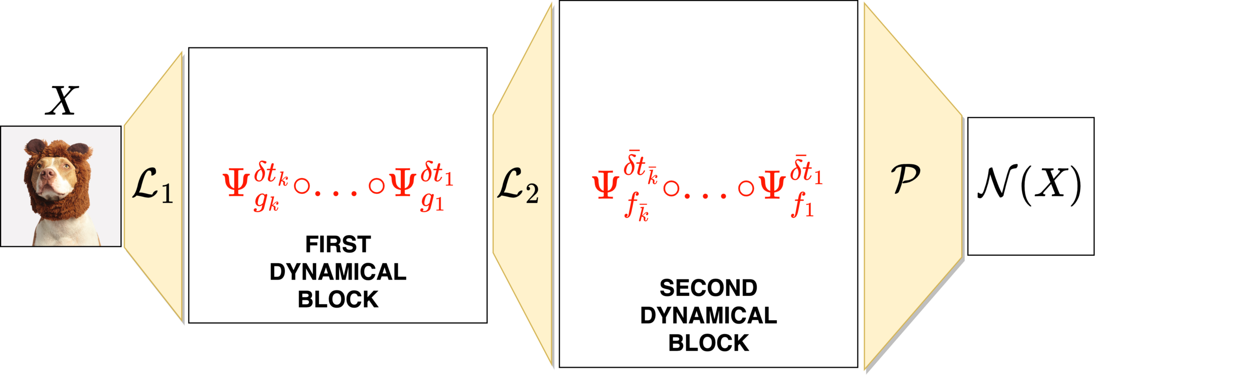
Defining neural networks with prescribed properties
Pixel-based learning
\(U^{n+1} = \Phi(U^n)\)
GOAL: Approximate the map \(\Phi\)
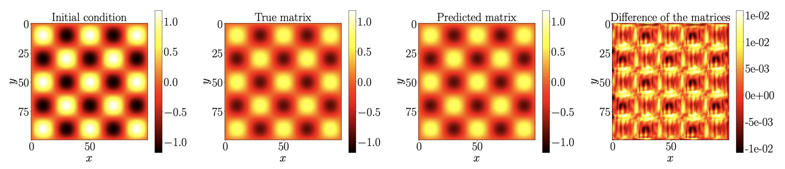
Predictions at time \(40\delta t\)
Fisher's equation:
\(\partial_t u=\alpha \Delta u+u(1-u)\)
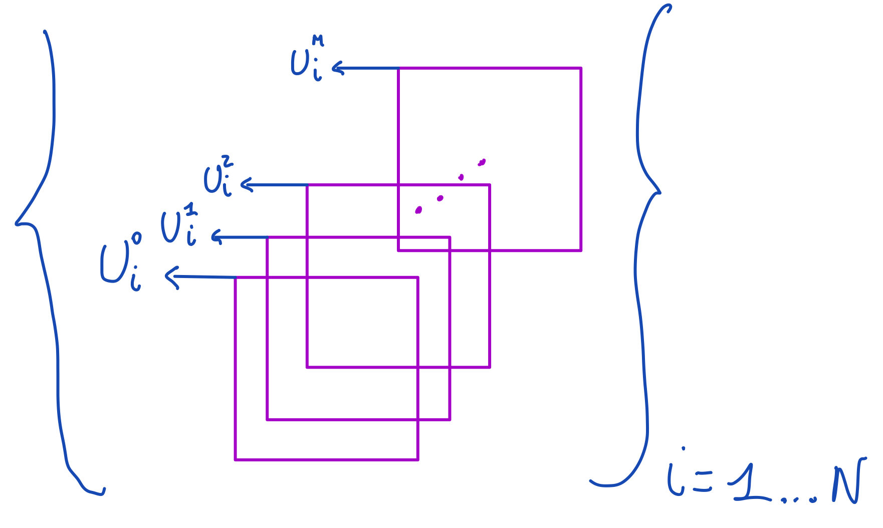
Approximation of space-time dynamics of PDEs
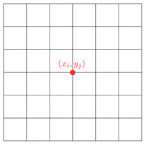
\(0=t_0 < t_1<...<t_M\)
\(U_{ij}^n = u(t_n,x_i,y_j)\)
{
Method of lines
Initial PDE
Semidiscretisation in space with finite differences
Approximation of the time dynamics
Method of lines
Initial PDE
Semidiscretisation in space with finite differences
Approximation of the time dynamics
Method of lines
Initial PDE
Semidiscretisation in space with finite differences
Approximation of the time dynamics
Finite differences as convolutions
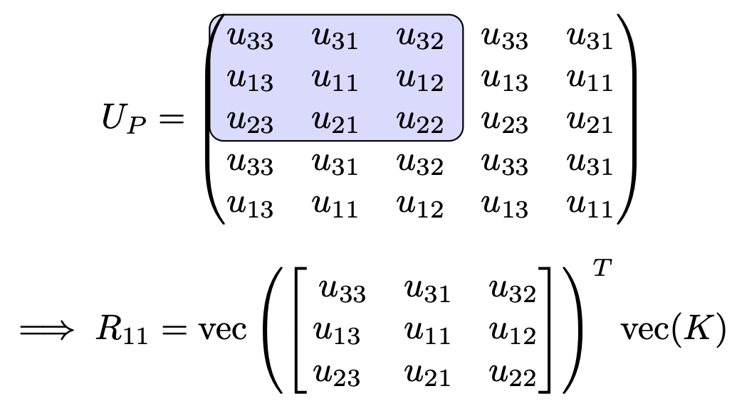
Example
Error splitting
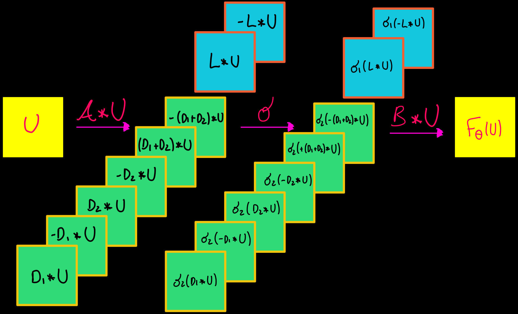
Layer of a ResNet we want to study
Splitting:
Useful activation functions
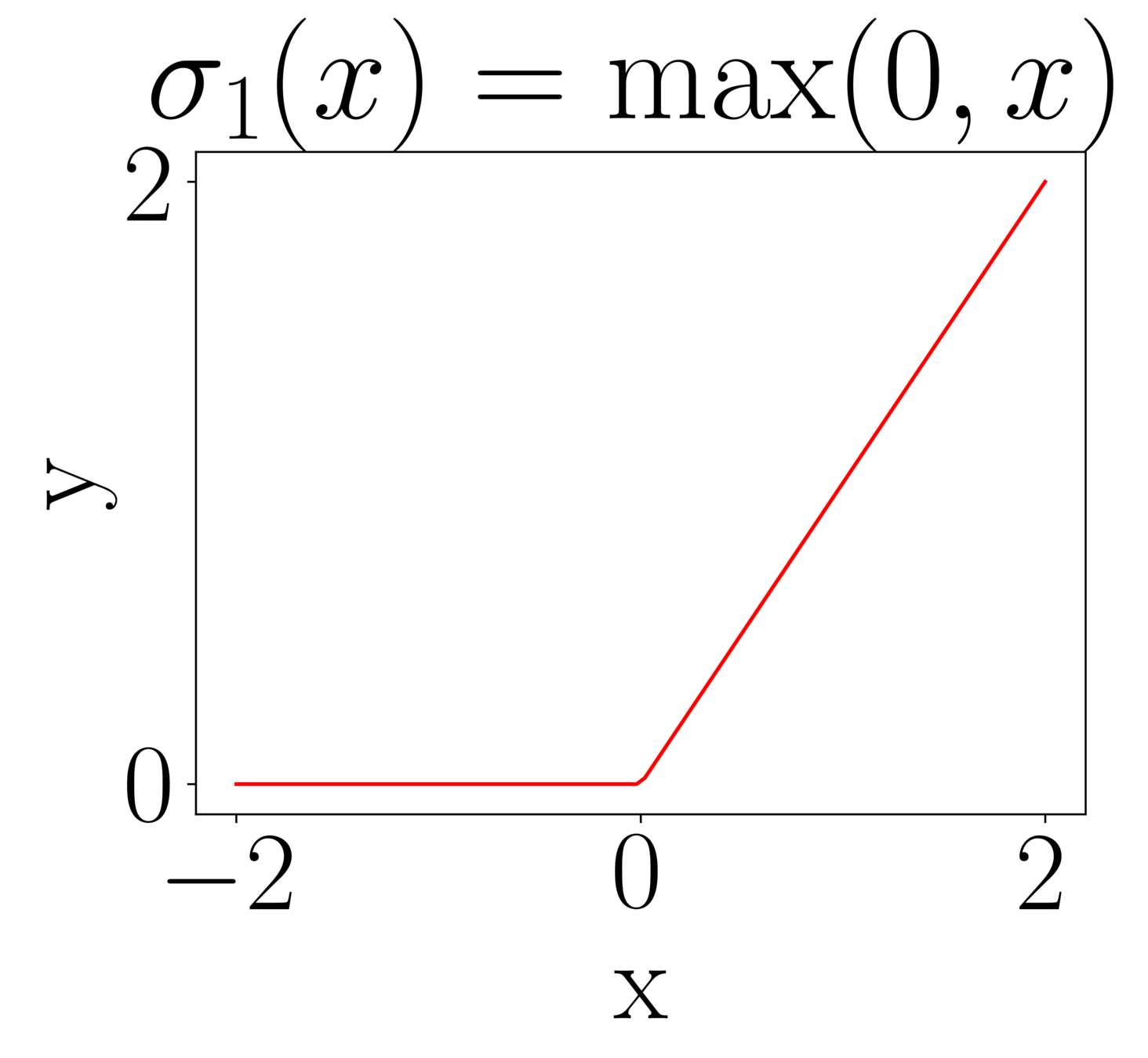
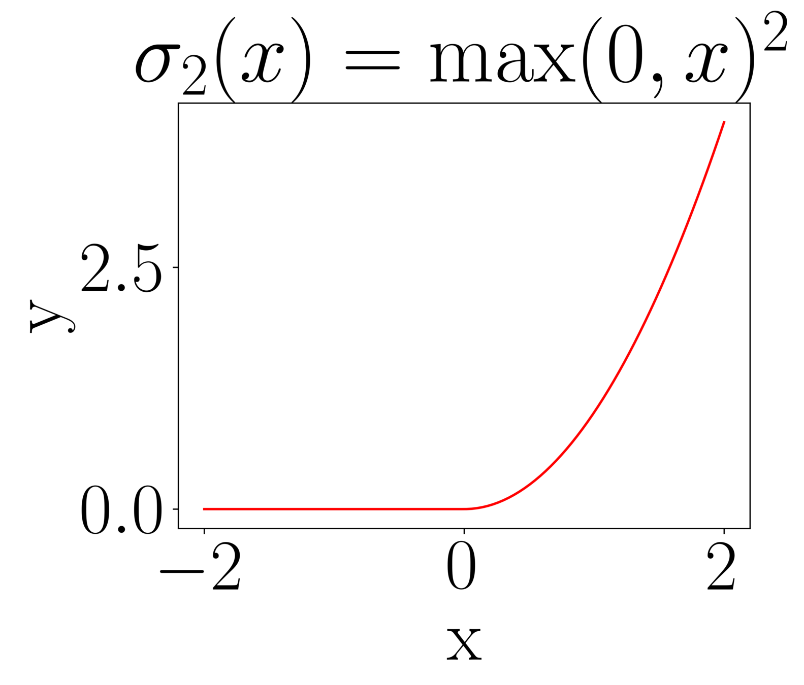
Simple but useful property:
\(x^p = \max(0,x)^p + (-1)^p\max(0,-x)^p\)
Approximation theorem
Simplified setting
Approximation theorem
Approximation theorem
This can theoretically be 0. In practice, it depends on to the optimisation error.
Examples of problems with a specific structure
What if I want a network to satisfy a certain property?
GENERAL IDEA
EXAMPLE
Property \(\mathcal{P}\)
\(\mathcal{P}=\) Volume preservation
Family \(\mathcal{F}\) of vector fields that satisfy \(\mathcal{P}\)
\(F_{\theta}(x,v) = \begin{bmatrix} \Sigma(Av+a) \\ \Sigma(Bx+b) \end{bmatrix} \)
\(\mathcal{F}=\{F_{\theta}:\,\,\theta\in\mathcal{P}\}\)
Integrator \(\Psi^{\delta t}\) that preserves \(\mathcal{P}\)
What if I want a network to satisfy a certain property?
GENERAL IDEA
EXAMPLE
Property \(\mathcal{P}\)
\(\mathcal{P}=\) Volume preservation
Family \(\mathcal{F}\) of vector fields that satisfy \(\mathcal{P}\)
\(F_{\theta}(x,v) = \begin{bmatrix} \Sigma(Av+a) \\ \Sigma(Bx+b) \end{bmatrix} \)
\(\mathcal{F}=\{F_{\theta}:\,\,\theta\in\mathcal{P}\}\)
Integrator \(\Psi^{\delta t}\) that preserves \(\mathcal{P}\)
What if I want a network to satisfy a certain property?
Choice of dynamical systems
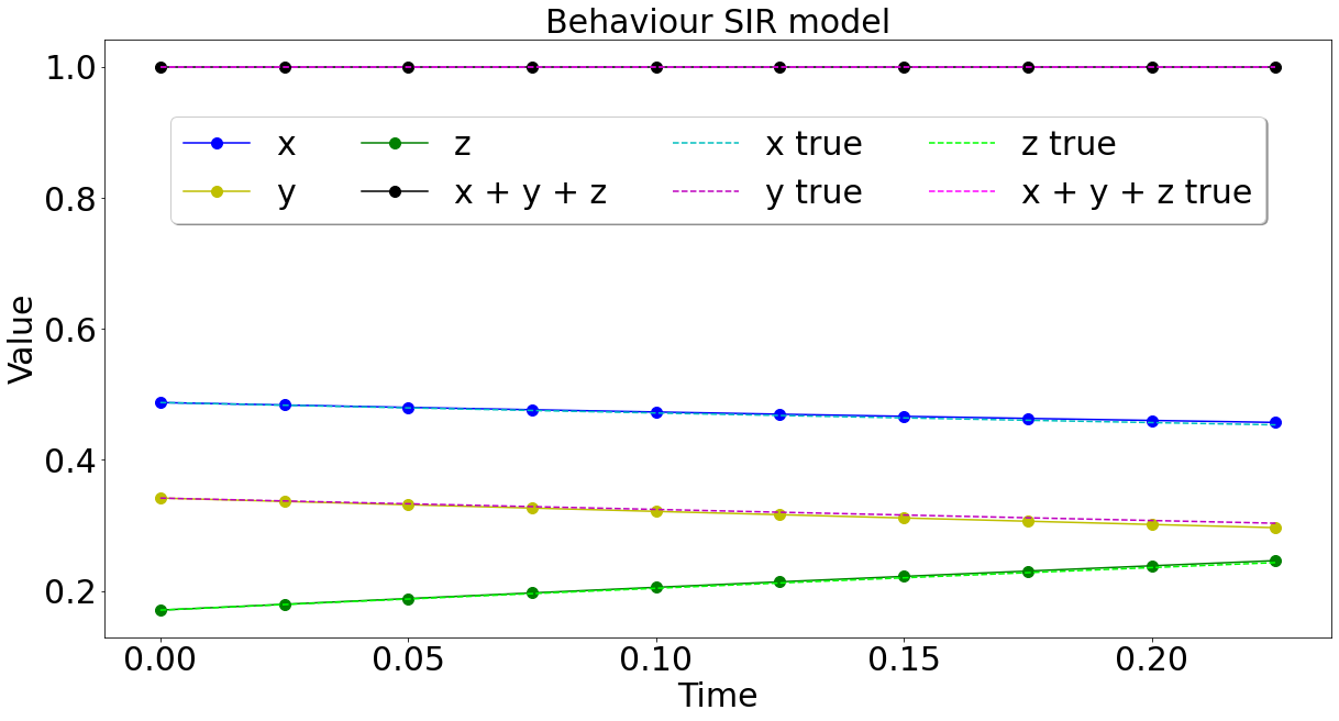
MASS-PRESERVING NEURAL NETWORKS
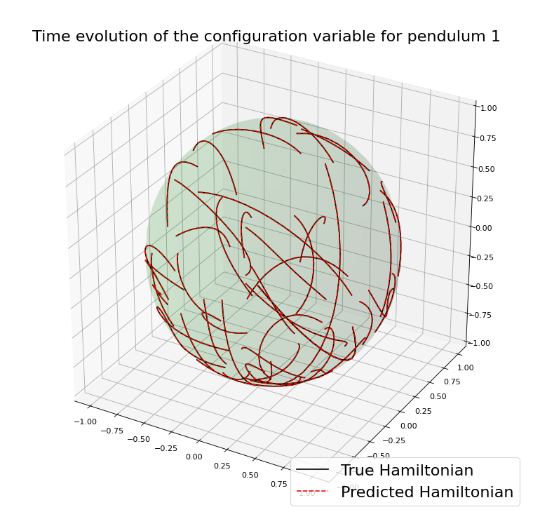
SYMPLECTIC NEURAL NETWORKS
Choice of dynamical systems
MASS-PRESERVING NEURAL NETWORKS
SYMPLECTIC NEURAL NETWORKS
Choice of numerical methods
MASS-PRESERVING NEURAL NETWORKS
SYMPLECTIC NEURAL NETWORKS
Any Runge-Kutta method
Any Symplectic numerical method
Choice of numerical methods
MASS-PRESERVING NEURAL NETWORKS
SYMPLECTIC NEURAL NETWORKS
Any Runge-Kutta method
Any Symplectic numerical method
Can we still approximate many functions?
Then \(F\) can be approximated arbitrarily well by composing flow maps of gradient and sphere preserving vector fields.
Presnov Decomposition
Idea of the proof
Thank you for the attention
- Celledoni, E., Jackaman, J., M., D., & Owren, B., preprint (2023). Predictions Based on Pixel Data: Insights from PDEs and Finite Differences.
- Celledoni, E., M. D., Owren B., Schönlieb C.B., Sherry F, preprint (2022). Dynamical systems' based neural networks
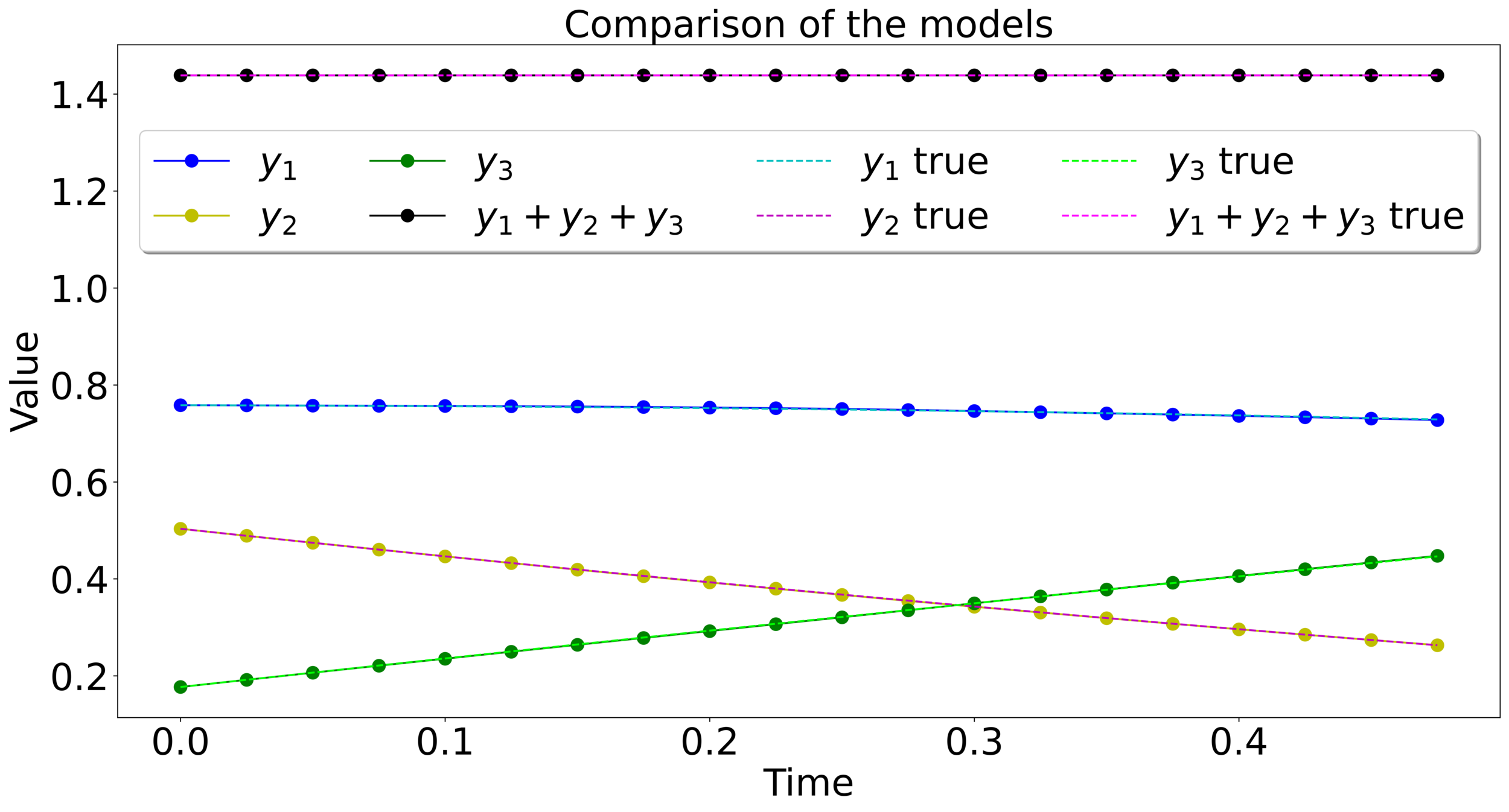
Mass-preserving networks
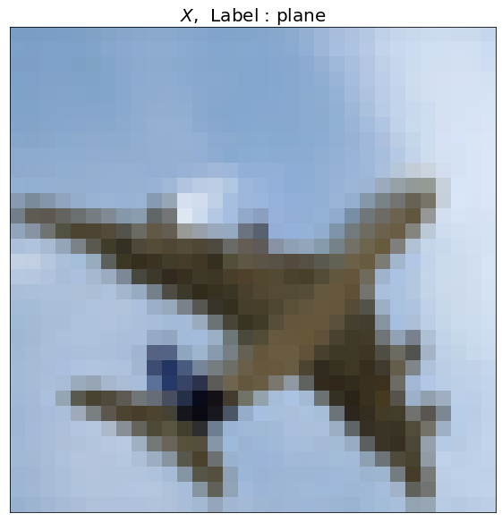
\(X\) , Label : Plane
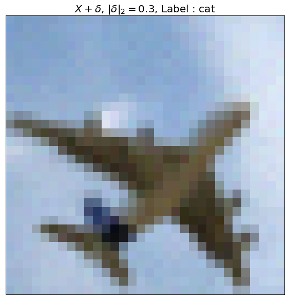
\(X+\delta\), \(\|\delta\|_2=0.3\) , Label : Cat
Adversarial robustness
Lipschitz-constrained networks
We impose :
Lipschitz-constrained networks
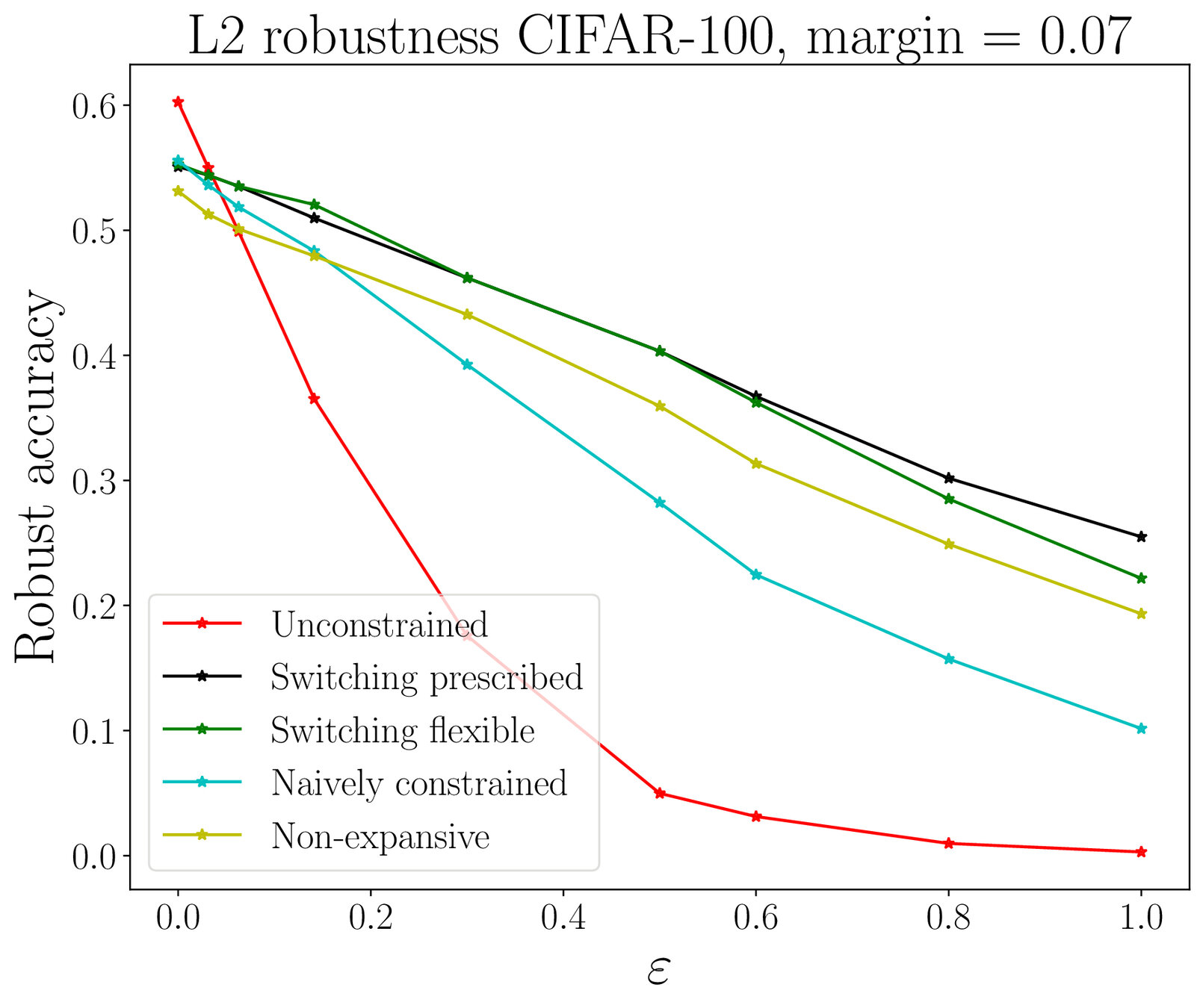
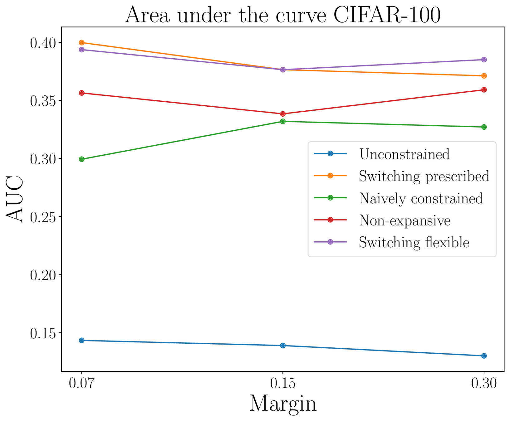
Adversarial robustness