Predictions Based on
Pixel Data
Davide Murari
davide.murari@ntnu.no

In collaboration with : Elena Celledoni, James Jackaman, Brynjulf Owren
TES Conference on Mathematical Optimization for Machine Learning
Pixel-based learning

\(U_i^{n+1} = \Phi^{\delta t}(U_i^n)+\delta_i^j\)
Predictions at time \(40\delta t\)
Fisher's equation:
\(\partial_t u=\alpha \Delta u+u(1-u)\)
DATA: \(\{(U_i^0,U_i^1,...,U_i^M\}_{i=1,...,N}\)
Definition of the goal
\(\mathcal{F}\)
\(\mathcal{C}^0\)
\(\Phi^{\delta t}\)
\(f_{\theta}\)
Given 2-layer convolutional neural networks, defining the space \(\mathcal{F}\), we want to see how well \(\Phi^{\delta t}\) can be approximated by functions in \(\mathcal{F}\).
Is there a constructive way to realize that approximation?
Approximation of space-time dynamics of PDEs
{
\(0=t_0 < t_1<...<t_M\)
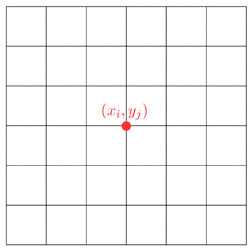
\((U^n)_{rs} = u(t_n,x_r,y_s)\)
\(x_r=r\delta x,\,\,y_s=s\delta x\)
Method of lines
Initial PDE
Method of lines
Initial PDE
Method of lines
Initial PDE
Semidiscretisation in space with finite differences
Method of lines
Initial PDE
Semidiscretisation in space with finite differences
Approximation of the time dynamics
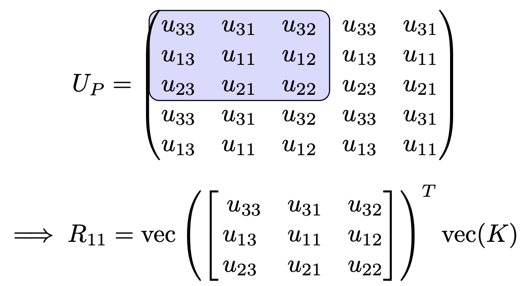
Finite differences as convolutions
Example
Error splitting
Layer of a ResNet we want to study
Splitting:
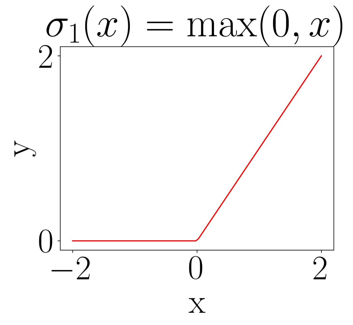
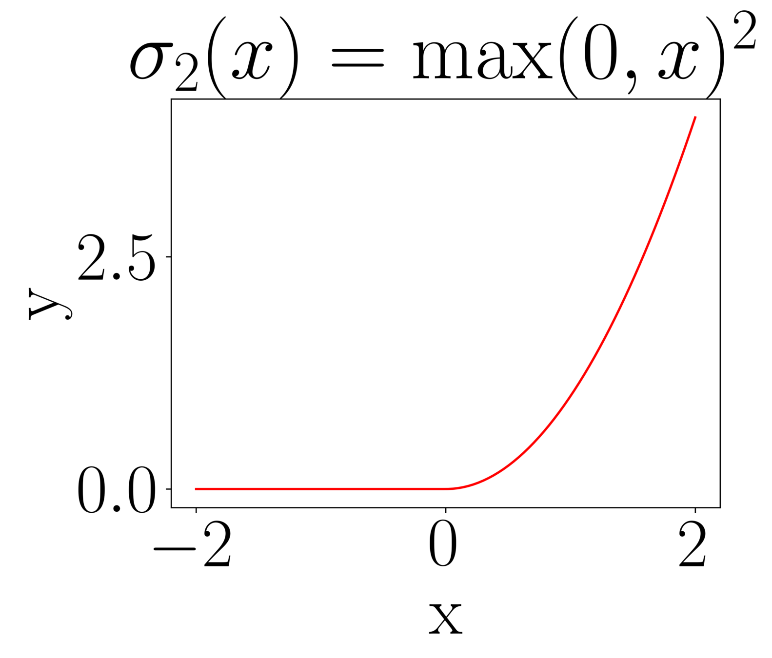
Useful activation functions
Simple but useful property:
\(x^p = \max(0,x)^p + (-1)^p\max(0,-x)^p\)
Approximation theorem
Simplified setting
Approximation theorem
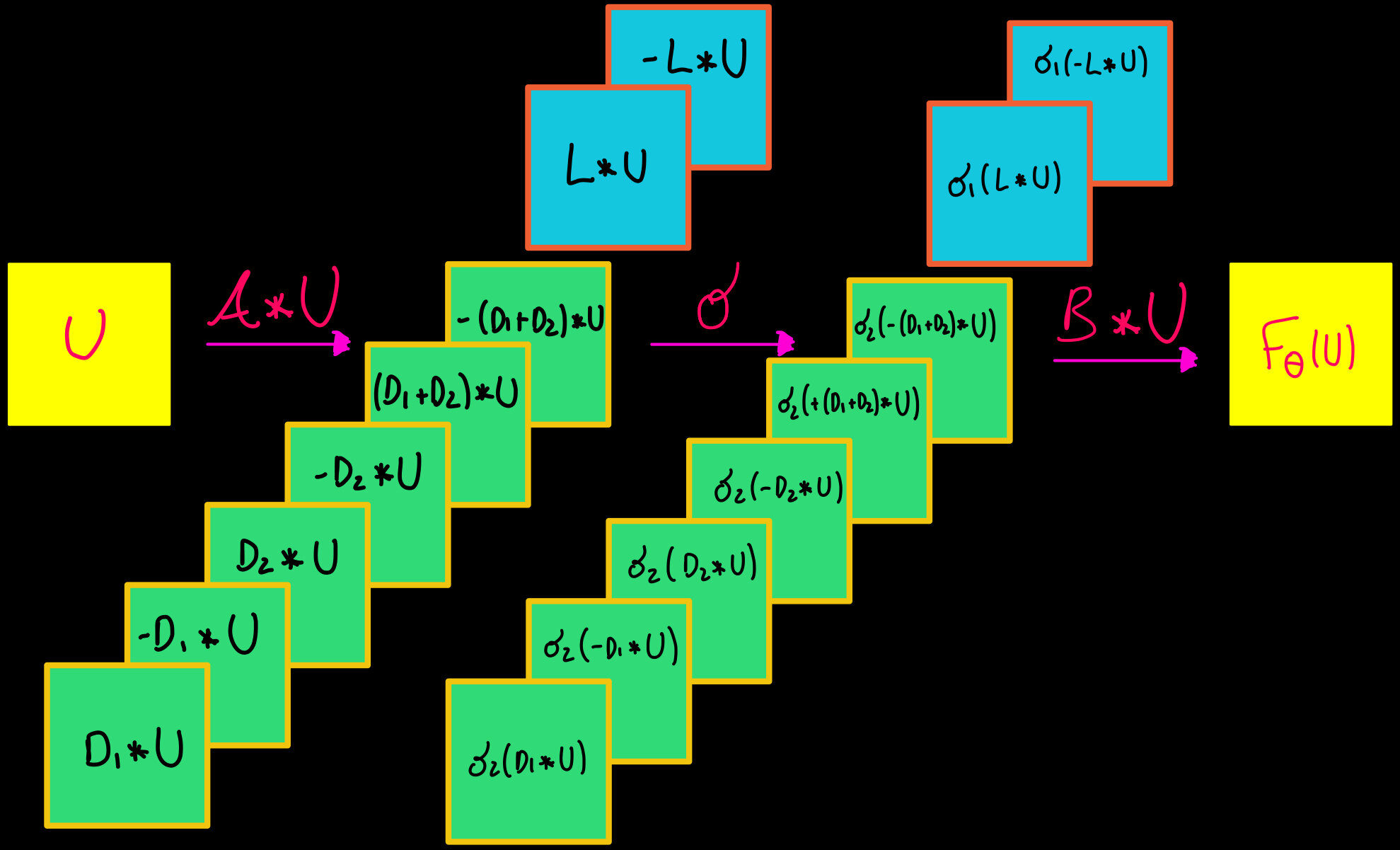
Approximation theorem
This can theoretically be 0. In practice, it depends on to the optimisation error.
This implies
Thank you for the attention
- Celledoni, E., Jackaman, J., M., D., & Owren, B., preprint (2023). Predictions Based on Pixel Data: Insights from PDEs and Finite Differences.