From neural networks to dynamical systems and back
Davide Murari
Talk at CIA seminar - 24/03/2023

\(\texttt{davide.murari@ntnu.no}\)
In collaboration with : Elena Celledoni, Andrea Leone, Brynjulf Owren, Carola-Bibiane Schönlieb and Ferdia Sherry
Neural networks
Dynamical
systems
- Approximating unknown vector fields
- Approximating solutions of ODEs
- Theoretical study of ResNets
- Designing ResNets with desired properties

Supervised learning
Consider two sets \(\mathcal{C}\) and \(\mathcal{D}\) and suppose to be interested in a specific (unknown) mapping \(F:\mathcal{C}\rightarrow \mathcal{D}\).
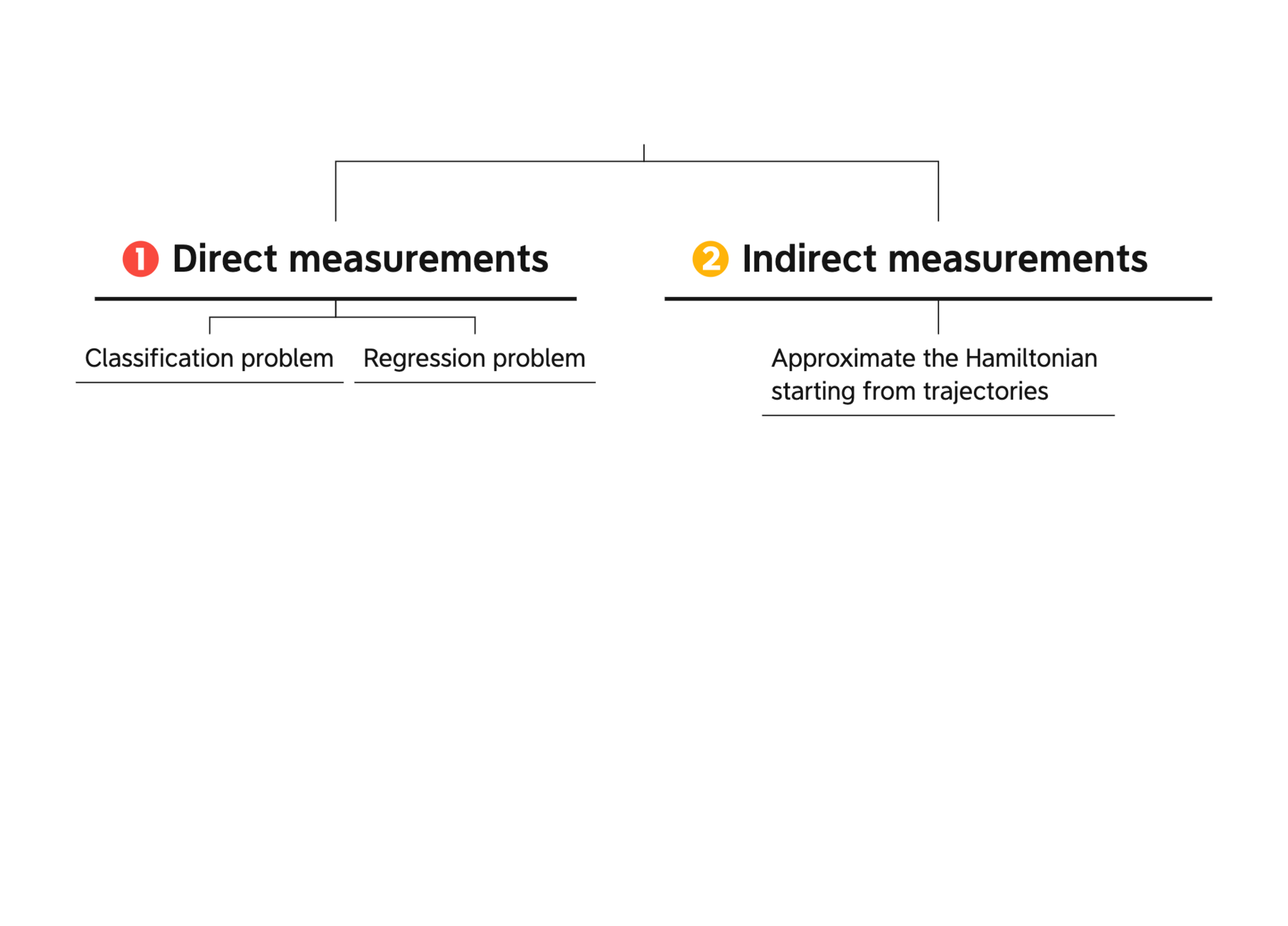
The data available can be of two types:
- Direct measurements of \(F\): \(\mathcal{T} = \{(x_i,y_i=F(x_i)\}_{i=1,...,N}\subset\mathcal{C}\times\mathcal{D}\)
- Indirect measurements that characterize \(F\): \(\mathcal{I} = \{(x_i,z_i=G(F(x_i))\}_{i=1,...,N}\subset\mathcal{C}\times G(\mathcal{D})\)
GOAL: Approximate \(F\) on all \(\mathcal{C}\).
(+ reproduce qualitative behaviour of \(F\) )
Examples of these tasks


What are neural networks
They are compositions of parametric functions
\( \mathcal{NN}(x) = f_{\theta_k}\circ ... \circ f_{\theta_1}(x)\)
Examples
\(f_{\theta}(x) = x + B\Sigma(Ax+b),\quad \theta = (A,B,b)\)
ResNets
Feed Forward
Networks
\(f_{\theta}(x) = B\Sigma(Ax+b),\quad \theta = (A,B,b)\)
\(\Sigma(z) = [\sigma(z_1),...,\sigma(z_n)],\quad \sigma:\mathbb{R}\rightarrow\mathbb{R}\)
Approximating Hamiltonians of constrained mechanical systems
- Celledoni, E., Leone, A., Murari, D., Owren, B., JCAM (2022). Learning Hamiltonians of constrained mechanical systems.
Definition of the problem
GOAL : approximate the unknown \(f\) on \(\Omega\)
DATA:
Approximation of a dynamical system
Introduce a parametric model
1️⃣
3️⃣
Choose any numerical integrator applied to \(\hat{f}_{\theta}\)
2️⃣
Choice of the model:
Unconstrained Hamiltonian systems
Unconstrained Hamiltonian systems
Choice of the model:
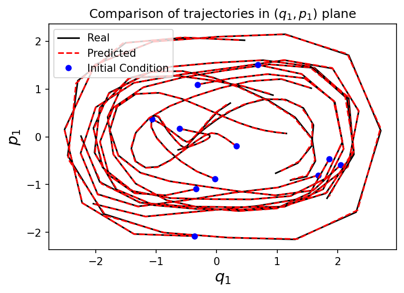
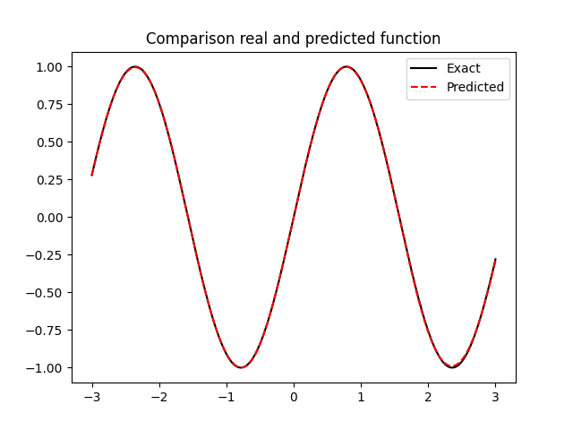
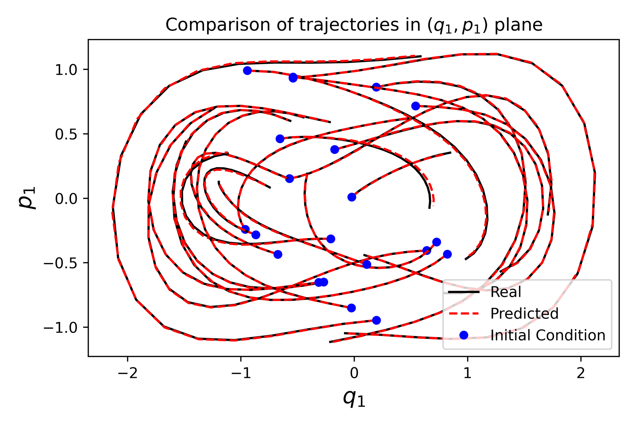
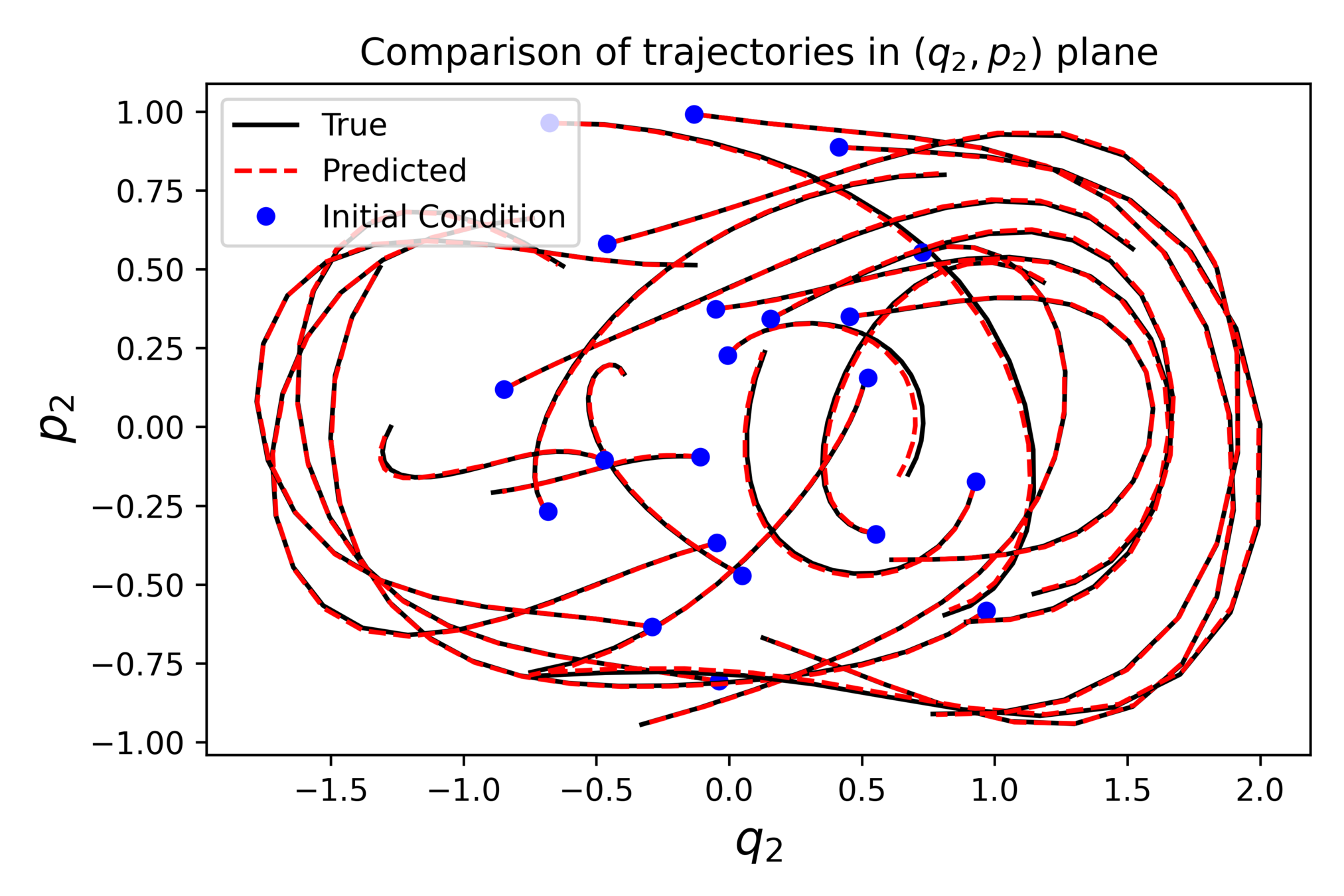
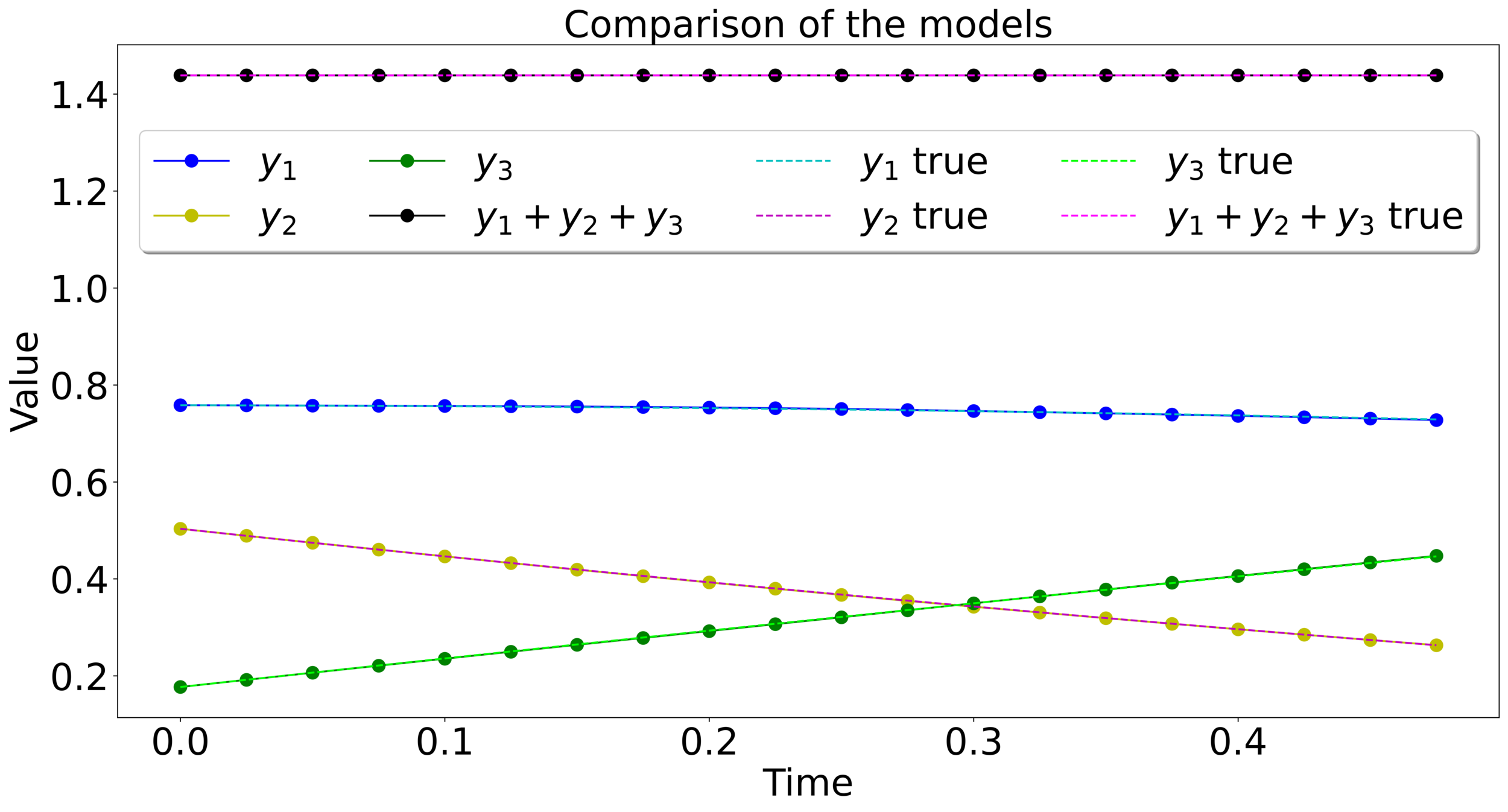
Measuring the approximation quality
Test initial conditions
Numerical experiment
⚠️ The integrator used in the test, can be different from the training one.
Physics informed regularization
If there is a known conserved quantity \(I(x(t))=I(x(0))\) we can add it to the loss, to get a physics informed regularization:
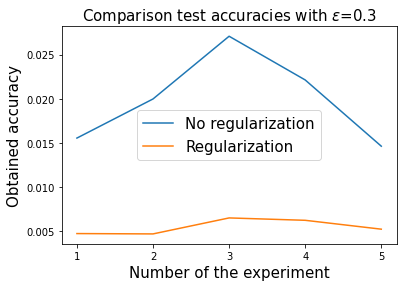
On clean trajectories
Constrained Hamiltonian systems
Modelling the vector field on \(\mathcal{M}\)
On \(\mathcal{M}\) the dynamics can be written as
⚠️ On \(\mathbb{R}^{2n}\setminus\mathcal{M}\) the vector field extends non-uniquely.
Example with \(\mathcal{Q}=S^2\)
On \(\mathcal{M}\) the dynamics can be written as
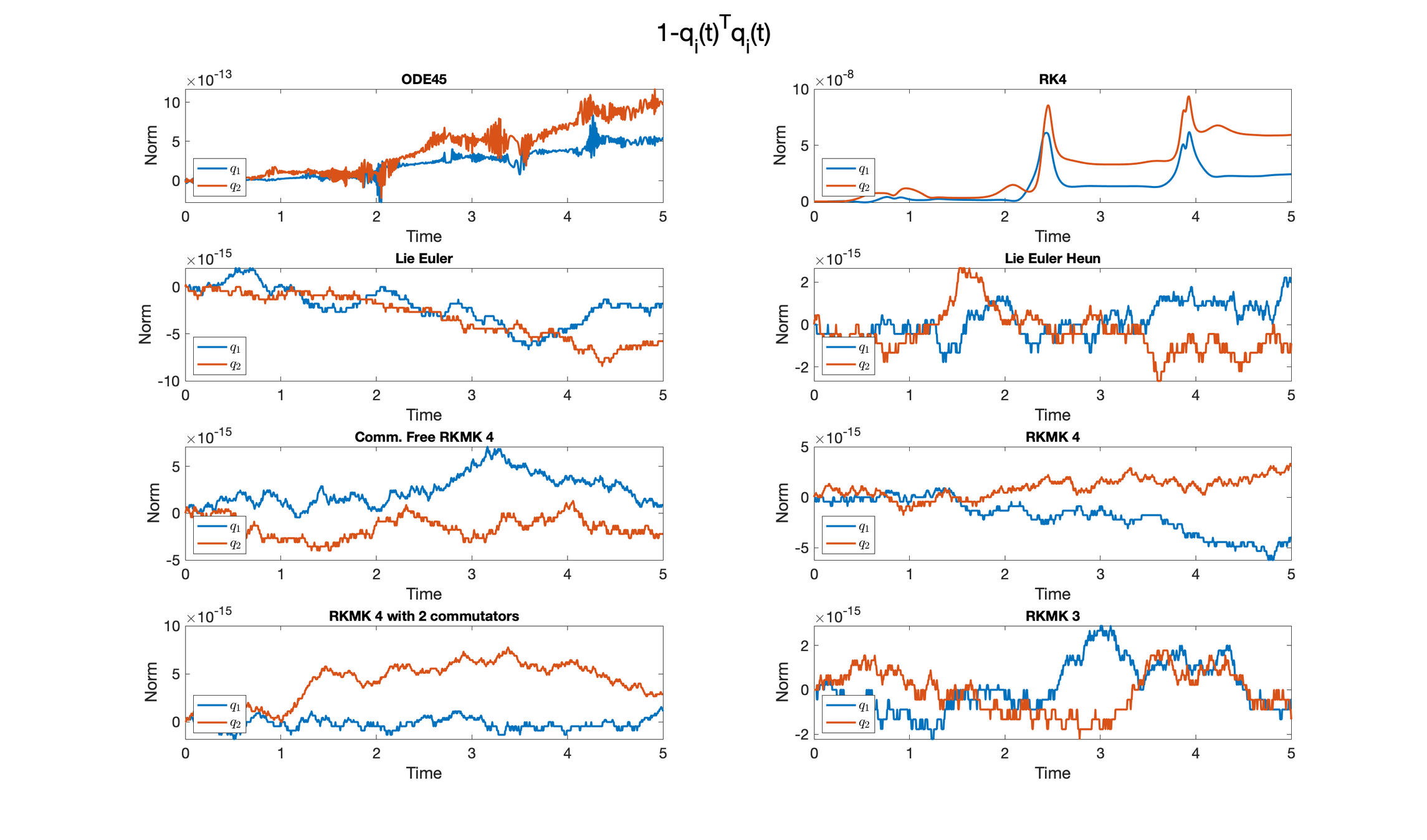
Learning constrained Hamiltonian systems
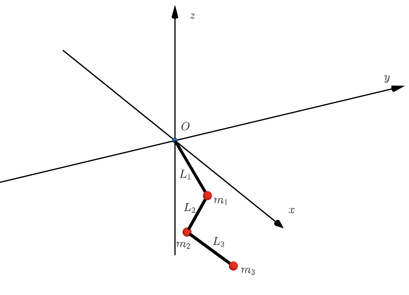
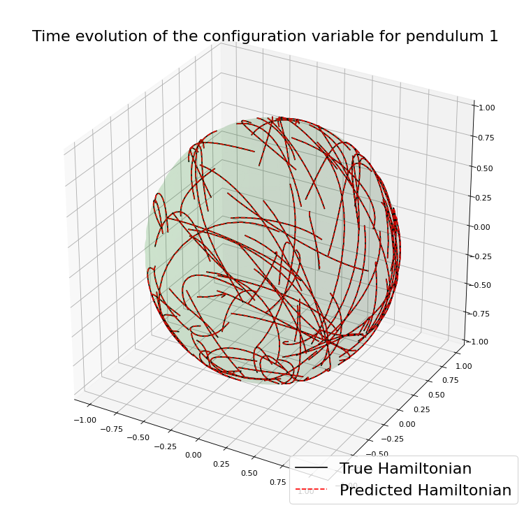
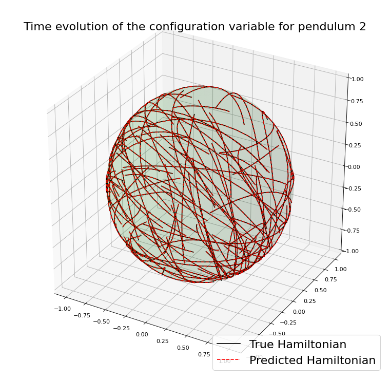
Chain of spherical pendula
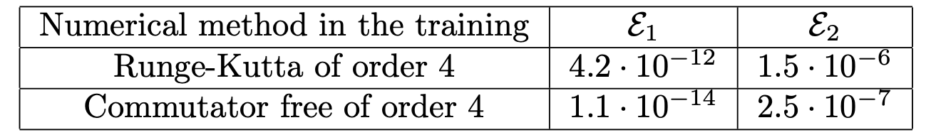
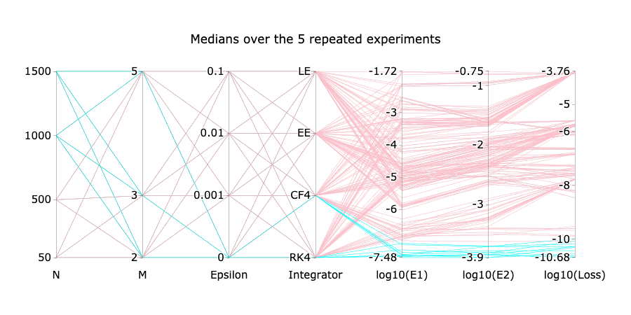
Choosing the numerical method for the training
Example with the double spherical pendulum
A case where preserving \(\mathcal{M}\) helps
Suppose to have just few unknown elements in the expression of the Hamiltonian
As a consequence, one expects a very accurate approximation.
Example with the spherical pendulum:
Similar results preserving \(\mathcal{M}\)
Designing and studying ResNets with dynamical systems' theory
- Celledoni, E., Murari D., Owren B., Schönlieb C.B., Sherry F, preprint (2022). Dynamical systems' based neural networks
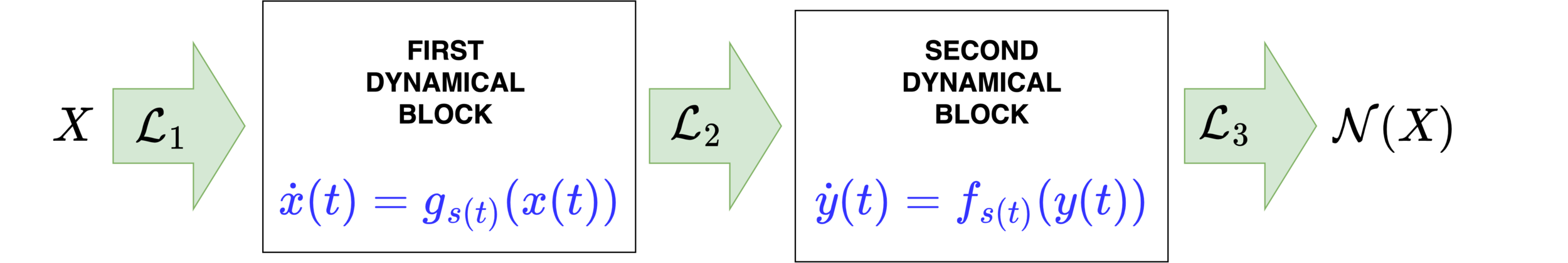
Neural networks motivated by dynamical systems
\( \mathcal{N}(x) = f_{\theta_M}\circ ... \circ f_{\theta_1}(x)\)
\( \dot{x}(t) = F(x(t),\theta(t))=:F_{s(t)}(x(t)) \)
Where \(F_i(x) = F(x,\theta_i)\)
\( \theta(t)\equiv \theta_i,\,\,t\in [t_i,t_{i+1}),\,\, h_i = t_{i}-t_{i-1}\)

Neural networks motivated by dynamical systems
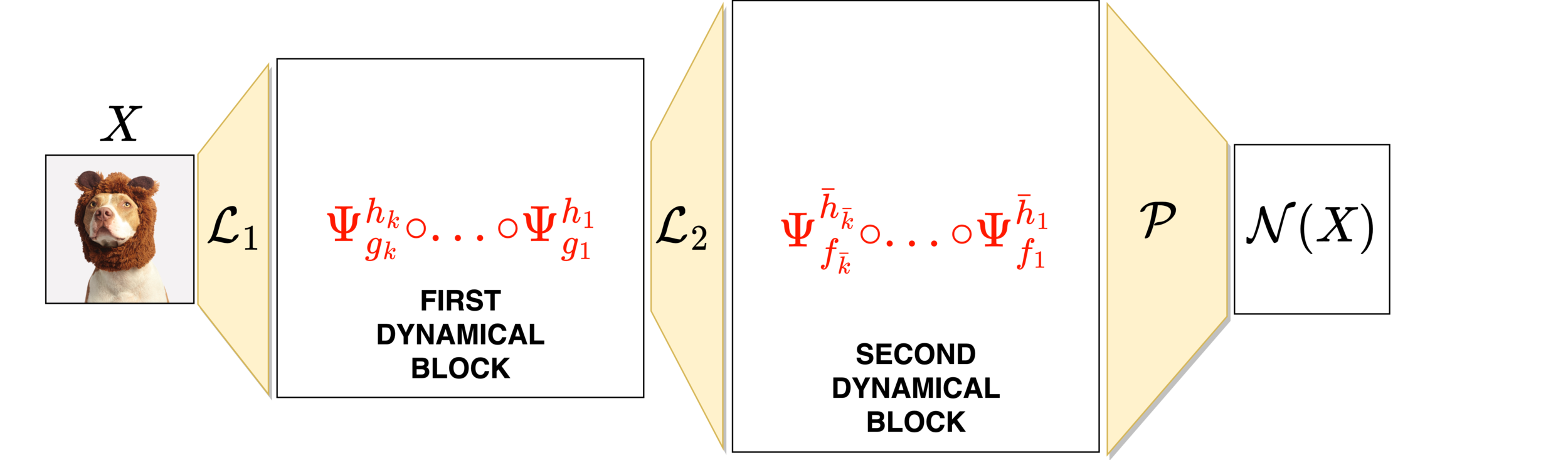
Neural networks motivated by dynamical systems
Accuracy is not all you need
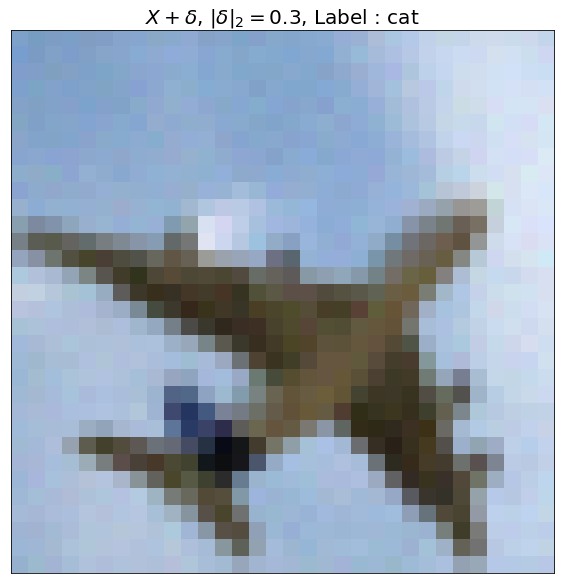
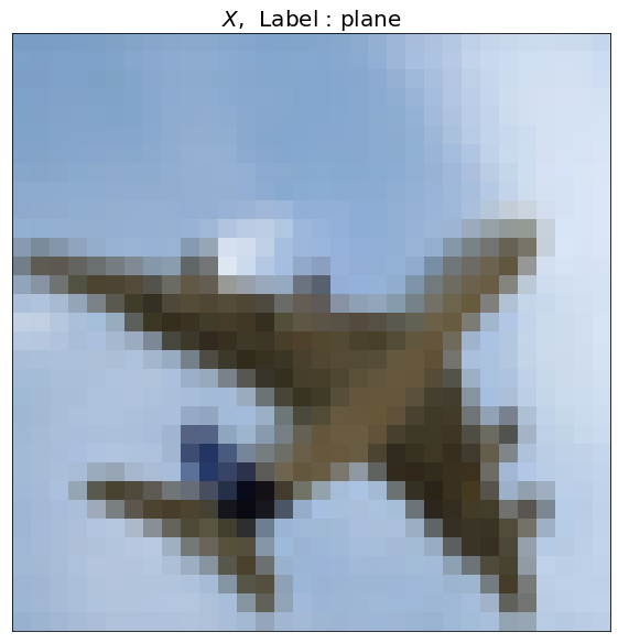
\(X\) , Label : Plane
\(X+\delta\), \(\|\delta\|_2=0.3\) , Label : Cat
GENERAL IDEA
EXAMPLE
Property \(\mathcal{P}\)
\(\mathcal{P}=\) Volume preservation
Family \(\mathcal{F}\) of vector fields that satisfy \(\mathcal{P}\)
\(F_{\theta}(x,v) = \begin{bmatrix} \Sigma(Av+a) \\ \Sigma(Bx+b) \end{bmatrix} \)
\(\mathcal{F}=\{F_{\theta}:\,\,\theta\in\mathcal{P}\}\)
Integrator \(\Psi^h\) that preserves \(\mathcal{P}\)
Imposing some structure
Examples
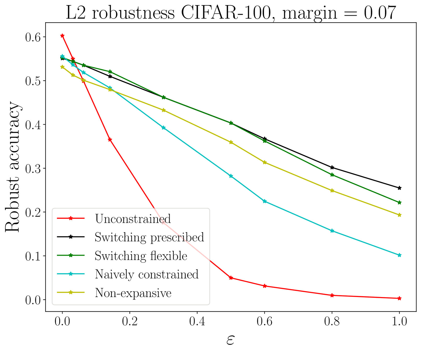
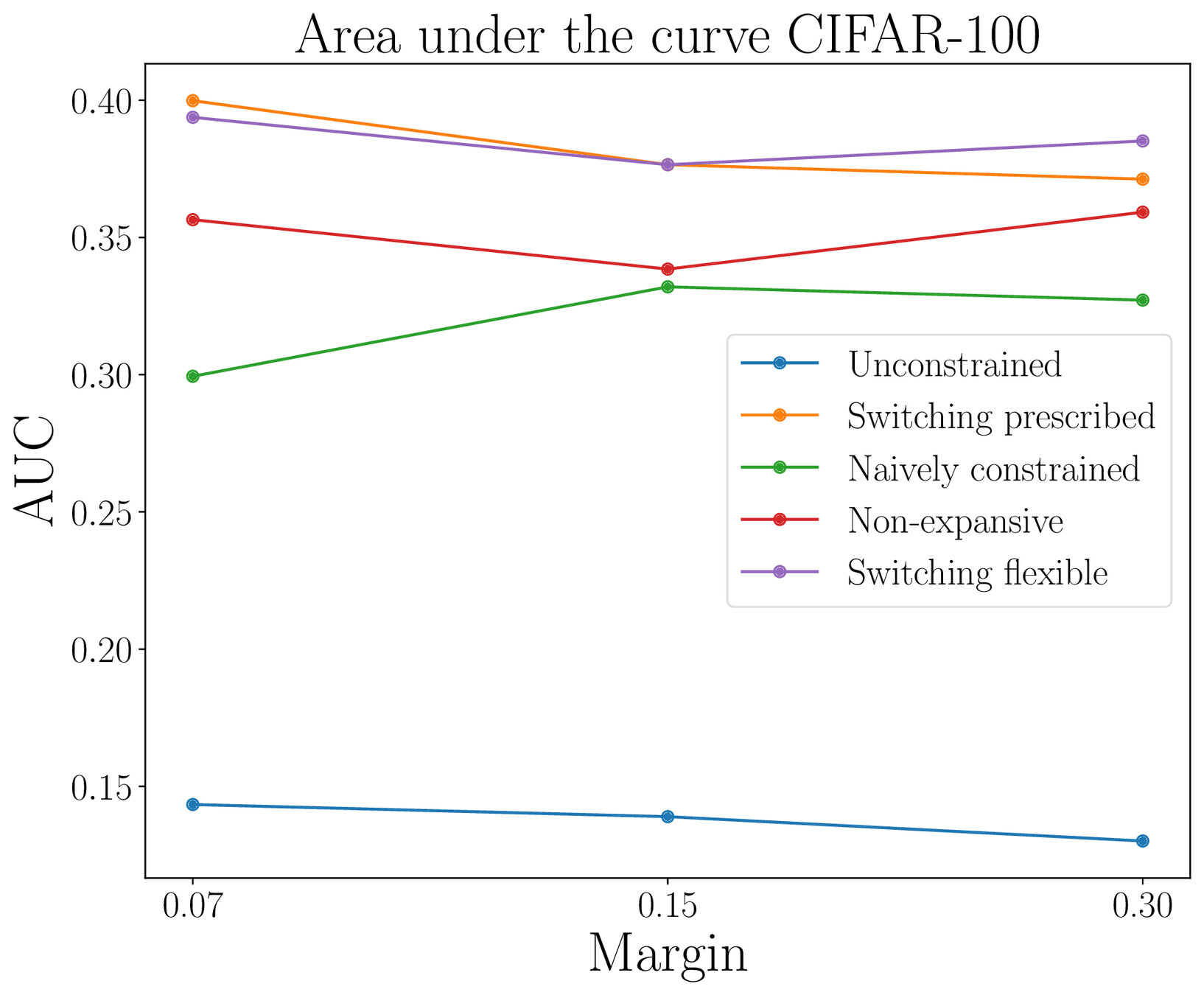
1-LIPSCHITZ NETWORKS
HAMILTONIAN NETWORKS
VOLUME PRESERVING, INVERTIBLE
Mass-preserving networks
Lipschitz-constrained networks
\(m=1\)
\(m=\frac{1}{2}\)
\(\Sigma(x) = \max\left\{x,\frac{x}{2}\right\}\)
Lipschitz-constrained networks
We impose :
Lipschitz-constrained networks
Adversarial robustness
Thank you for the attention
Case with \(\mathcal{M}\) homogeneous
A manifold \(\mathcal{M}\) is homogeneous if there is a Lie group \(\mathcal{G}\) that defines a transitive group action \(\varphi:\mathcal{G}\times\mathcal{M}\rightarrow\mathcal{M}\).
A vector field \(f\) on \(\mathcal{M}\) can be represented as \(f(x) = \varphi_*(\xi(x))(x)\), for a function
\(\xi:\mathcal{M}\rightarrow\mathfrak{g}\simeq T_e\mathcal{G}\).
Lie Group Methods are a class of methods exploiting this structure and preserving \(\mathcal{M}\). The simplest is Lie Euler:
\(y_i^{j+1} = \varphi(\exp(\Delta t \,\xi(y_i^j)),y_i^j)\)
Basic idea of a class of Lie group methods
\(\mathcal{M}\)
\(y_i^j\)
\(y_i^{j+1}=\varphi_g(y_i^j)\)
\(\mathfrak{g}\)
\(\xi\)
\(\exp\)
\(\mathcal{G}\)
\(\varphi_g\)
\(\Psi^{\Delta t}\)
\(0\)
\(\Delta t \xi(y_i^j)\)
\(g=\exp(\Delta t\,\xi(y_i^j))\)
\(f\in\mathfrak{X}(M)\)
\(f^L\in\mathfrak{X}(\mathfrak{g})\)