Dealing with resampling-induced errors
when estimating the activity

in clinical multi-imaging

Davide Poggiali (PNC)

In coll. w/: Stefano De Marchi (DM)

Diego Cecchin (DIMED).

DWCAA21 - Sept. 6th, 2021

Summary:

Motivation
Interpolation for image resampling
Bounding the error
Gibbs Effect in image resampling
Fake Nodes for image oversampling
Conclusions

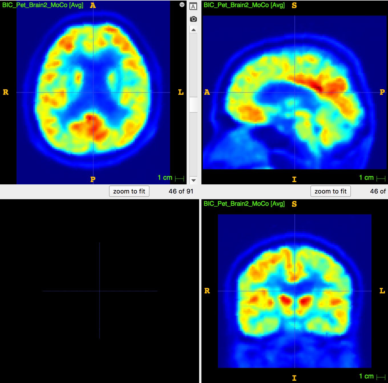
1. Motivation: Sampling problem in PET/MRI

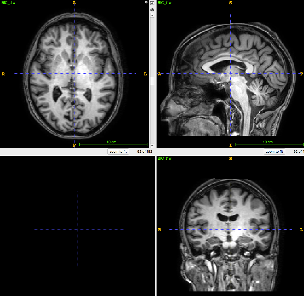
3D T1-weighted MRI:

usually ~1 mm $^3$ voxel

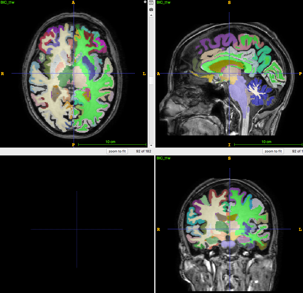
Segmentation/parcellation at full resolution

PET image:

usually ~8mm $^3$ voxel

How to apply segmentation?

1. Undersampling T1 segmentation

2. Upsampling PET image

3. PET segmentation (no MRI)

Sampling problem in PET/MRI

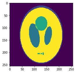
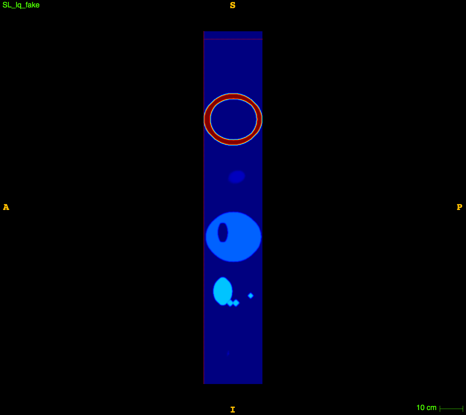
In silico test: Shepp-Logan 3D Phantom

Using a phantom the gold standard is known and we can analyse the errors of approximation.

High resolution "morphological" image

Segmentation mask

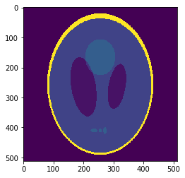
Low resolution "functional" image

Resampling is performed in ANTs

https://github.com/ANTsX/ANTs

Original values at masks (gold standard):

g=[0.0, 1.0, 0.05, 0.3, 0.15, 0.2]

1mm^3

8mm^3

1mm^3

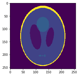
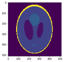
Downsampled segmentation mask

Low resolution "functional" image

Undersampling segmentation

The 2-norm relative error is $\sqrt{\sum{ (g_i-v_i)^2 \over g_i^2}}\approx 0.058$

Sampled mean values at masks:

v =[0.00033, 0.937, 0.0523, 0.298, 0.153, 0.206]

8mm^3

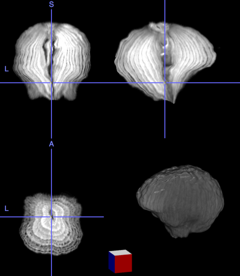
Oversampled "functional" image

Oversampling functional image

The 2-norm relative error is ~$0.103$

Segmentation mask

Sampled mean values at masks:

v=[0.0015, 0.889, 0.054, 0.297, 0.158, 0.209]

1mm^3

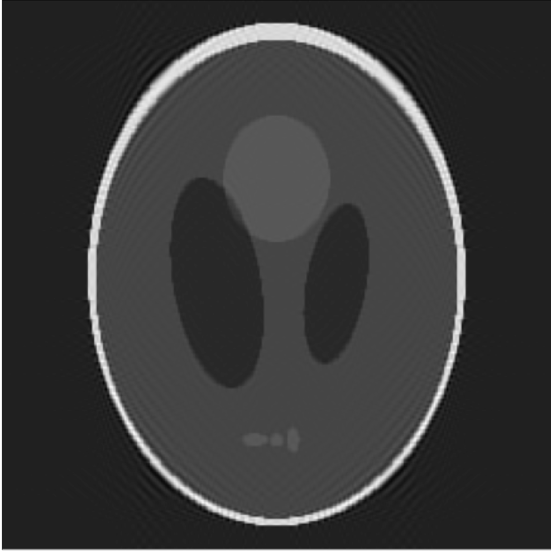
If we look at the pointwise interpolation error

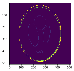
We can observe it is mostly higher distributed around the borders, where the gradient is higher.

This is what we call the Gibbs Effect.

2. Interpolation for image resampling

A three-dimesional MRI can be ~ $10^8$ voxels (256x256x256 takes ~800Mb in double precision, uncompressed) and counting. Hence a fast, lightweight interpolation method is needed.

Q: What is the fastest interpolation method?

R: When the interpolation and evaluation nodes coincide 😛😛😛😛

2. Interpolation for image resampling

Let us take a $10^8$ voxels image. The interpolation matrix would be $10^8 \times 10^8$ .... ~80Pb in double precision!

What is the fastest (nontrivial) interpolation method?

Choose a basis;
Compute Interpolation/Evaluation matrices;
Solve a linear system;
Multiply Eval. matrix by coefficients.

2. Interpolation for image resampling

So we need to choose a basis:

Separable → the interpolation is computed on each axis sequentially;
Cardinal → no need to compute or invert the Interpolation matrix;
Compact supported → Evaluation matrix is sparse.

To achieve that we have to suppose that the interpolation nodes are on a equispaced grid.

2. Interpolation for image resampling

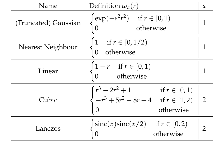
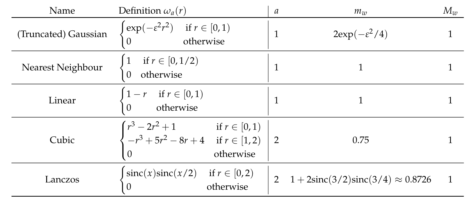
[Step I] Let $\omega_a: \mathbb{R}_+ \to \mathbb{R}$, with $a\in\mathbb{N}$ the support radius, a function such that:

$\omega_a(0) = 1$;
$\omega_a(k) = 0\;\; \forall~ k \in \mathbb{N}\setminus \{0\}$;
$\omega_a(r) = 0\;\;\forall~ r \geq a$.

2. Interpolation for image resampling

[Step II] Let $\{t_i\}$, a set of $N$ equispaced points of the interval $[\alpha, \beta]$. Then we define for the univariate basis

\[ w_{\sigma}(t - t_i)=\frac{\omega_a(\sigma|t-t_i|)}{\sum_{j=0}^N \omega_a(\sigma |t-t_j|)},\]
with $\sigma = \frac{N}{\beta-\alpha}$ a scaling factor.

2. Interpolation for image resampling

[Step III] The three-variate interpolant is

\[\mathcal{P}_f (\bm{x}) = \sum_{ijk} f(\bm{x}_{ijk})W_{ijk}(\bm{x})\]

with

\[W_{ijk}(x, y, z) = w_{\sigma_1}(x-x_i)\; w_{\sigma_2}(y-y_i) \;w_{\sigma_3}(z-z_i)\]

the separable basis. This basis is also:

Cardinal;
Compact supported;
Radial in each component.

This is called interpolation by convolution.

3. Bounding the error

Being the basis separable we can consider univariate interpolation

Let us suppose without loss of generality that the function
\[f:[0,1] \to \mathbb{R}\]
is known at $x_i = \frac{i}{N},\;\;i=0,\ldots,N$.

By using a function $\omega_a(r)$ satisfying (I), we define the interpolating function
\[ \mathcal{P}^N_f(x) = \sum_{i=0}^N w(x-x_i) f(x_i)\]

with $w(t - t_i) = \frac{\omega_a(\frac{1}{N}|t-t_i|)}{\sum_{j=0}^N \omega_a(\frac{1}{N} |t-t_j|)}$.

3. Bounding the error

Lemma: Suppose that $x\in (x_k, x_{k+1})$ for some $k\in 0, \ldots, N-1$ and that the support radius is $a\in\mathbb{N}$.

Then
$$\mathcal{P}^N_f(x) = \sum_{i=\max(0, k-a)}^{\min(N, k+a-1)} w(x-x_i) f(x_i).$$

3. Bounding the error

Theorem [Pointwise error bound]: If the interpolation point $x\in(x_k, x_{k+1})$ with $a\leq k \leq N-a+1$ and $m_{w}>0$, then

\[|\mathcal{P}^N_f (x) - f(x)| \leq \frac{M_{w}}{m_{w}} \sum_{i=k-a}^{k+a-1} |f(x) - f(x_i)|.\]

Once calculated

\[M_{w} = \max_{x\in [0,1]} \left| \omega_a(N|x-x_i|)\right|,\;\;\text{and}\]

\[m_{w} = \min_{x\in [0,1]} \left|\sum_{j=0}^N \omega_a(N|x-x_j|) \right|\]

we can formulate

3. Bounding the error

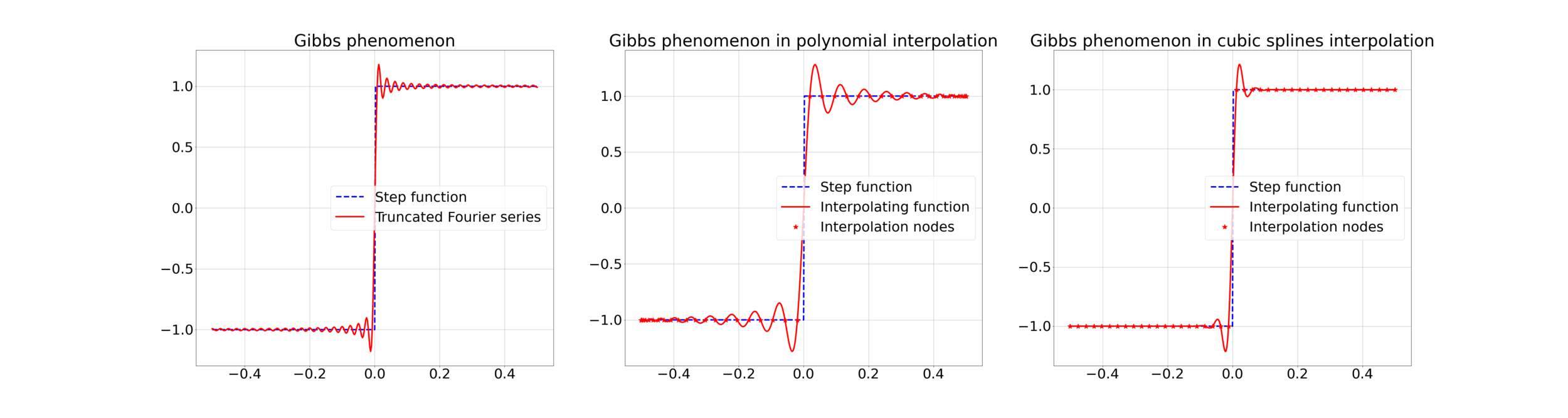
4. Gibbs effect in Image Resampling

Gibbs effect (in a nutshell):

Appears at discontinuities as oscillatory;
Does not vanish as $N\to\infty$;
As $N\to\infty$ their frequency grows, the amplitude reaches a plateau.

4. Gibbs effect in Image Resampling

Gibbs effect is called "ringing effect" in MRI.

4. Gibbs effect in Image Resampling

Corollary 1: if $f$ is continuous in $x\in[0,1]$, then
\[\lim_{N\to\infty} |\mathcal{P}^N_f (x) - f(x)| = 0 .\]

Corollary 2: if $f$ is discontinuous at $x\in[0,1]$, and the limit of the error exists, then
\[0 \leq \lim_{N\to\infty} |\mathcal{P}^N_f (x) - f(x)| \leq a\frac{M_{w}}{m_{w}} |f(x^-) - f(x^+)| .\]

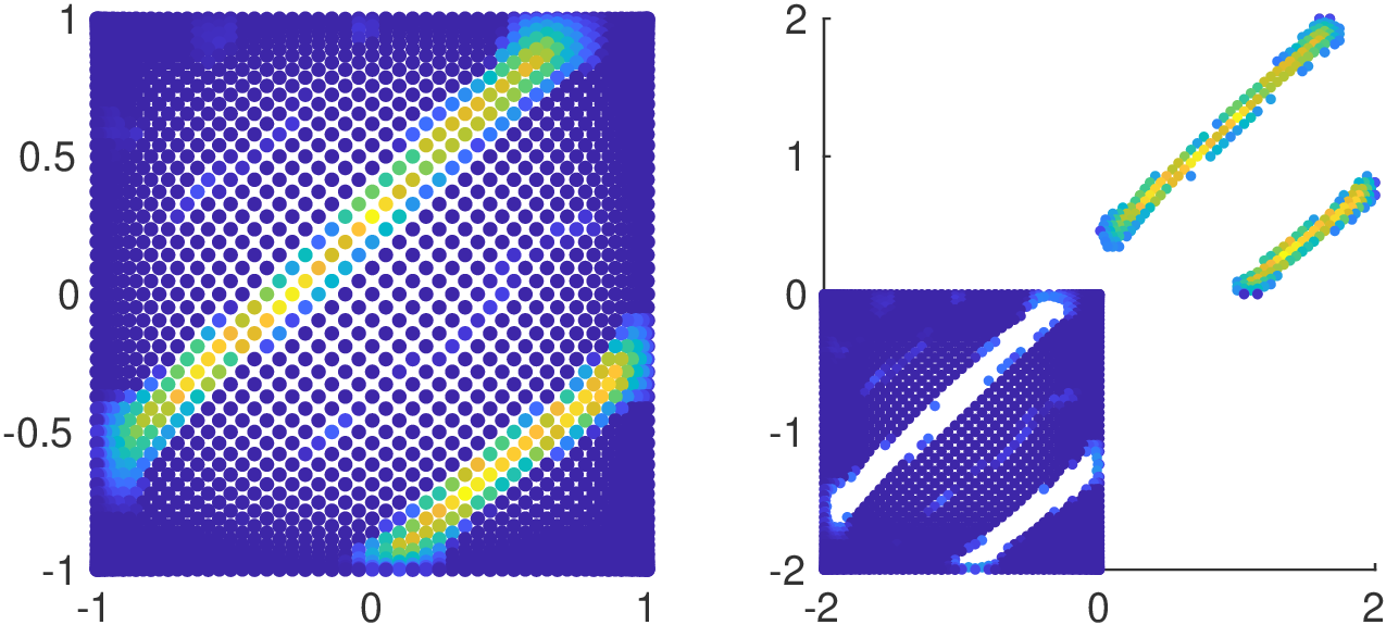
5. Fake Nodes for image oversampling

Interpolation on Fake Nodes, or interpolation via Mapped Bases is a technique that applies to any interpolation method. It has shown in many cases the ability of obtaining a better interpolation without getting new samples.

In terms of code: suppose that you have a generic interpolation function ...

def my_fancy_interpolator(x,y,xx):
  .......
  .......
  return yy

def my_fancy_interpolator(x,y,xx):
  p = np.polyfit(x,y)
  yy = np.polyval(p,xx)
  return yy

instead of calling the function directly you define a mapping function S and interpolate over the fake nodes S(x)

f = lambda x: np.log(x**2+1)
x = np.linspace(-1,1,10)
y = f(x)
xx = np.linspace(-1,1,100)



yy = my_fancy_interpolator(x,y,xx)

f = lambda x: np.log(x**2+1)
x = np.linspace(-1,1,10)
y = f(x)
xx = np.linspace(-1,1,100)

S = lambda x: -np.cos(np.pi * .5 * (x+1))

yy = my_fancy_interpolator(S(x),y,S(xx))

5. Fake Nodes for image oversampling

In other words, given a function

f: \Omega \subseteq \mathbb{R}^d \longrightarrow \mathbb{R}\;\;\;\;\; {d \in \mathbb{N}},

a set of distinct nodes

X = \{ x_0, \dots, x_N\} \subset \Omega,

and a set of basis functions

\mathcal{B} = \{ b_i: \Omega \longrightarrow \mathbb{R} \}_{i = 0, \ldots, N}

The interpolant is given by a function

\displaystyle \mathcal{P}(\bm{x}) = \sum_{i=0}^{N} c_i b_i(\bm{x})

s.t.

\mathcal{P}(\bm{x}_i)=y_i:=f(\bm{x}_i) \;\;\forall i

\mathcal{B} = \{ b_i \circ S: \Omega \longrightarrow \mathbb{R}^d \}_{i = 0, \ldots, N}

\displaystyle \mathcal{R}^s(\bm{x}) = \sum_{i=0}^{N} c_i b_i(S(\bm{x}))

\mathcal{R}^s(\bm{x}_i)=y_i:=f(\bm{x}_i) \;\;\forall i

5. Fake Nodes for image oversampling

This process can be seen equivalently as:

1. Interpolation over the mapped basis

\[\mathcal{B}^s = \{b_i \circ S \}_{i=0, \dots, N}.\]

2. Interpolation over the original basis $\mathcal{B}$ of a function $g: S(\Omega) \longrightarrow\mathbb{R}$

at the fake nodes

\[S(X) = \{S(x_i) \}_{i=0, \dots, N}.\]

$g\in C^s$ must satisfy $g(S(x_i)) = f(x_i)\;\;\forall i$.

If $\mathcal{P} \approx g $ on $S(X)$ with the original basis,

then $\mathcal{R}^s = \mathcal{P} \circ S \approx f $ on $X$

5. Fake Nodes for image oversampling

To avoid Gibbs Effect the function $g$ is supposed to be as smooth as possible.

Moreover, in order to be applied to Interpolation by Convolution methods a regular grid is mandatory.

Hence we have to assign some values to the unmapped nodes of the regular grid.

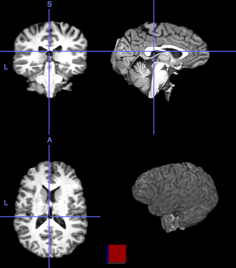
5. Fake Nodes for image oversampling

$(2mm)^3$

$1mm^3$

Fake image

5. Fake Nodes for image oversampling

In vitro validation:

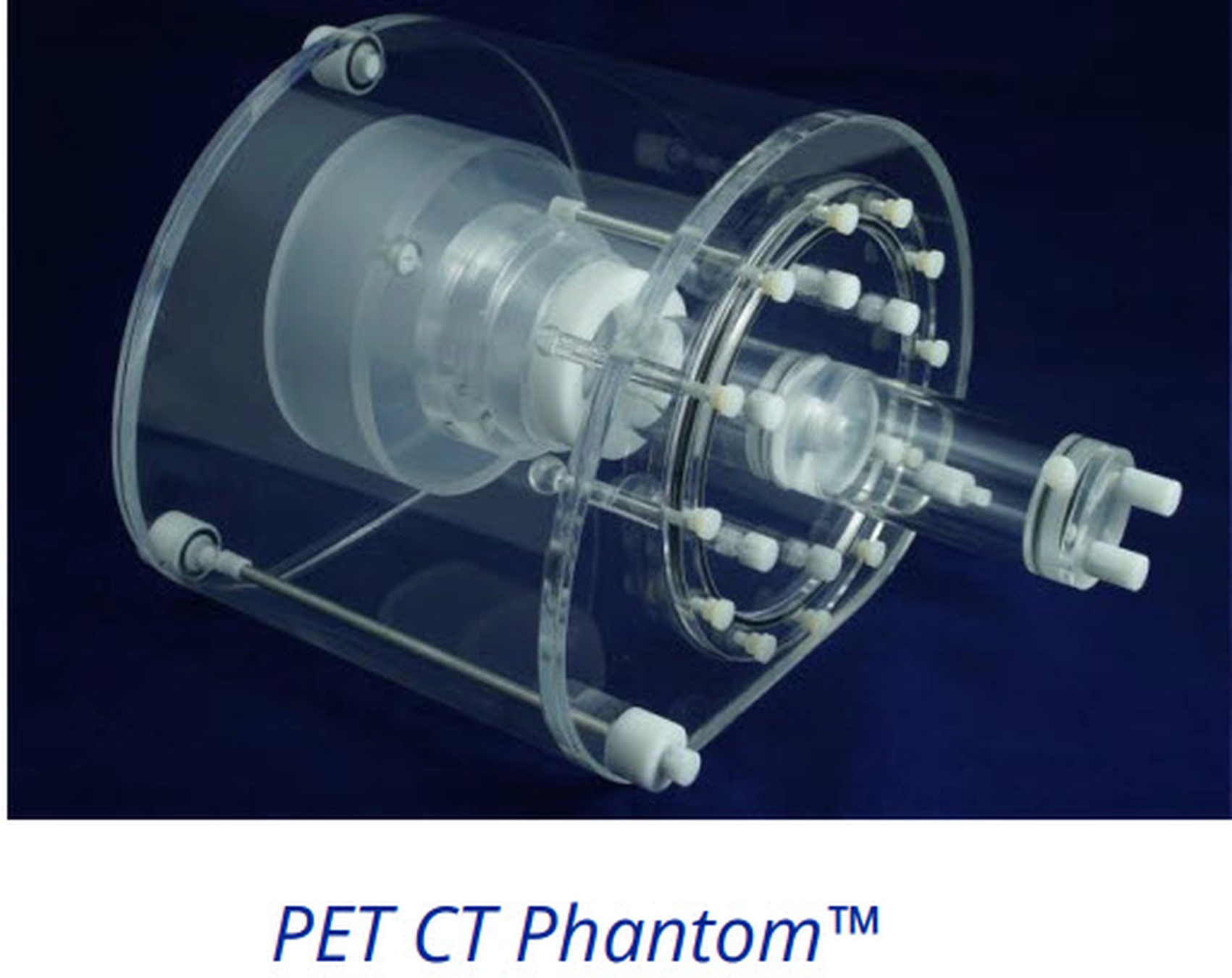
The RIDER PET/CT phantom images is a dataset of repeated scans of a dummy (20 scans of the same phantom).

Muzi, Peter, Wanner, Michelle, & Kinahan, Paul. (2015).
Data From RIDER_PHANTOM_PET-CT. The Cancer Imaging Archive.
http://doi.org/10.7937/K9/TCIA.2015.8WG2KN4W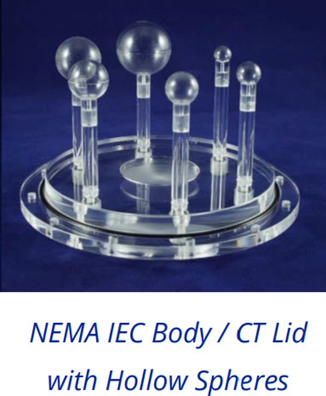

5. Fake Nodes for image oversampling

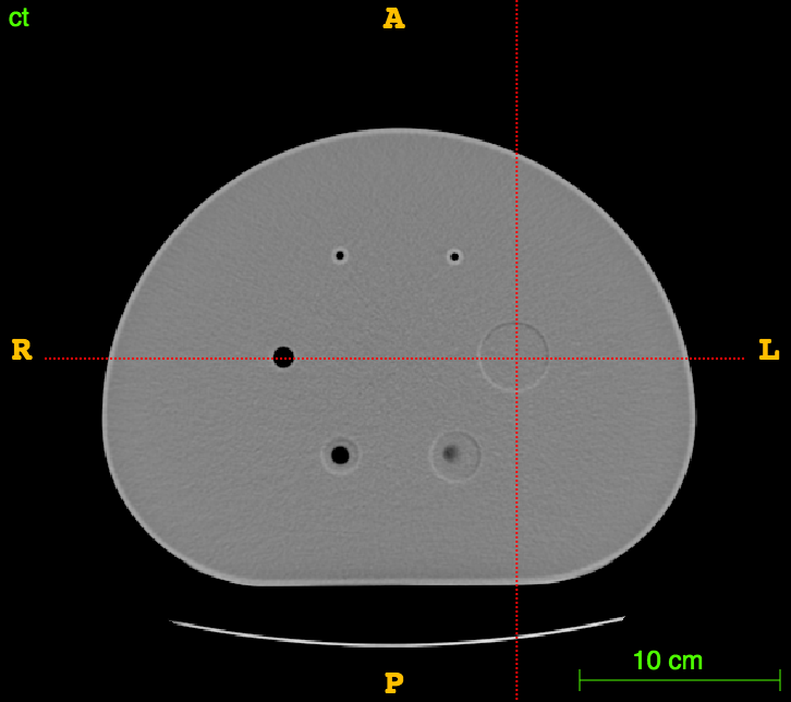
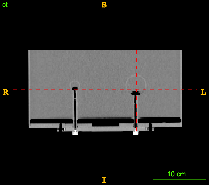
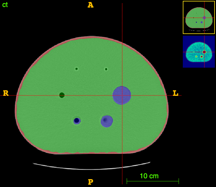
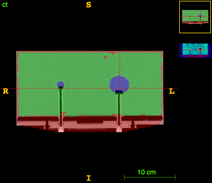
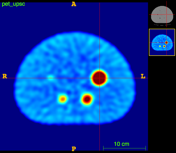
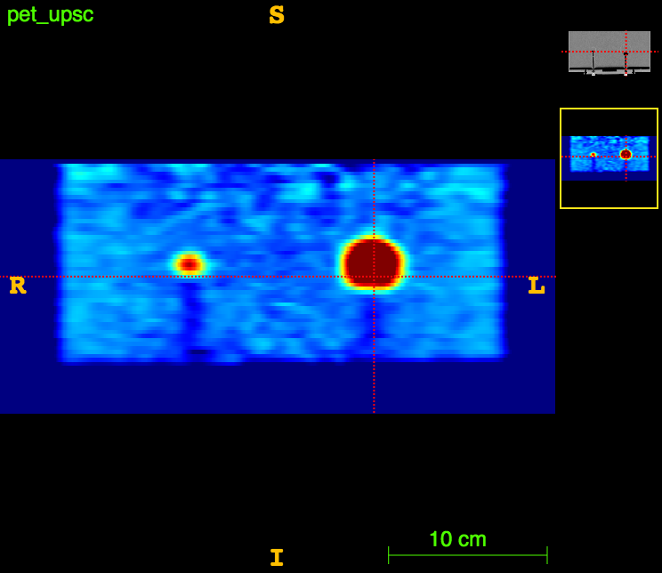
Axial

Sagittal

Axial

CT segm.

PET

5. Fake Nodes for image oversampling

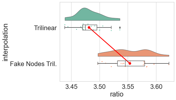
The ideal foreground/background ratio would be 4.

6. Conclusions

We have proven the presence of Gibbs effect in image oversampling;
We have proposed a Fake-Nodes based workaround in the context of Multimodal medical imaging;
We have evaluated such method both in silico and in vitro.

Future works:

Such approach might be extendable to generic imaging;
In the case of PET/[CT, MRI], the results are not that stunning, an exact PET quantification is still far from our hands.
Fake Nodes approach should be used in PET reconstruction.

References

[1] Burger, W., Burge, M.J., Principles of digital image processing: core algorithms; Springer, 2009.

[2] Dumitrescu, Boiangiu. A Study of Image Upsampling and Downsampling Filters. Computers doi:10.3390/computers8020030.4139

[3] S. De Marchi, F. Marchetti, E. Perracchione, Jumping with Variably Scaled Discontinuous Kernels (VSDKs), BIT Numerical Mathematics 2019.

[4] S. De Marchi, F. Marchetti, E. Perracchione, D. Poggiali, Polynomial interpolation via mapped bases without resampling, JCAM 2020.

[5] S. De Marchi, F. Marchetti, E. Perracchione, D. Poggiali, Multivariate approximation at Fake Nodes, AMC 2021.

[5] S. De Marchi, G. Elefante, E. Perracchione, D. Poggiali, Quadrature at Fake Nodes, DRNA 2021.
[6] C. Runge, Uber empirische Funktionen und die Interpolation zwischen aquidistanten Ordinaten, Zeit. Math. Phys, 1901.

[7] D. Poggiali, D. Cecchin, C. Campi, S. De Marchi, Oversampling errors in multimodal medical imaging are due to the Gibbs effect, doi:10.13140/RG.2.2.30924.13446/1

Thank you!

Dealing with resampling-induced errors when estimating the activity

in clinical multi-imaging

Summary:

1. Motivation: Sampling problem in PET/MRI

Sampling problem in PET/MRI

In silico test: Shepp-Logan 3D Phantom

2. Interpolation for image resampling

2. Interpolation for image resampling

2. Interpolation for image resampling

2. Interpolation for image resampling

2. Interpolation for image resampling

2. Interpolation for image resampling

3. Bounding the error

3. Bounding the error

3. Bounding the error

3. Bounding the error

4. Gibbs effect in Image Resampling

4. Gibbs effect in Image Resampling

4. Gibbs effect in Image Resampling

5. Fake Nodes for image oversampling

5. Fake Nodes for image oversampling

5. Fake Nodes for image oversampling

5. Fake Nodes for image oversampling

5. Fake Nodes for image oversampling

5. Fake Nodes for image oversampling

5. Fake Nodes for image oversampling

5. Fake Nodes for image oversampling

6. Conclusions

Dealing with resampling-induced errors
when estimating the activity