A Kinetic Neural Network Approach for Absolute Quantification and Change Detection in Positron Emission Tomography
D. Poggiali, postDoc
Roma, MASCOT18
Davide Poggiali, Diego Cecchin and Stefano De Marchi

Summary:
- Introduction
- Kinetics of the tracer in PET/MRI
- A new approach to kinetical modelling
- Results
- Conclusions & future works

What is PET/MRI?

1. Introduction
Motivation: The PET Grand Challenge 2018

Dataset:
- 5 simulated PET/MRIs
- dynamic PET images
- pre and post intervention
- unknown tracer
Aim:
"to identify areas and magnitude of receptor binding changes in a PET radioligand neurotransmission study"
2. Kinetics of the tracer in PET/MRI
Tracer kinetics is studied with ODE compartment model

A compartment is a set of tissues that exchanges energy/material to another set of tissues at the same rate

A classical example: Sokoloff model (1970s)
Absolute Metabolic rate:
General compartmental model formulation
Solution of the general model
in case
else
3. A new approach to kinetical modelling
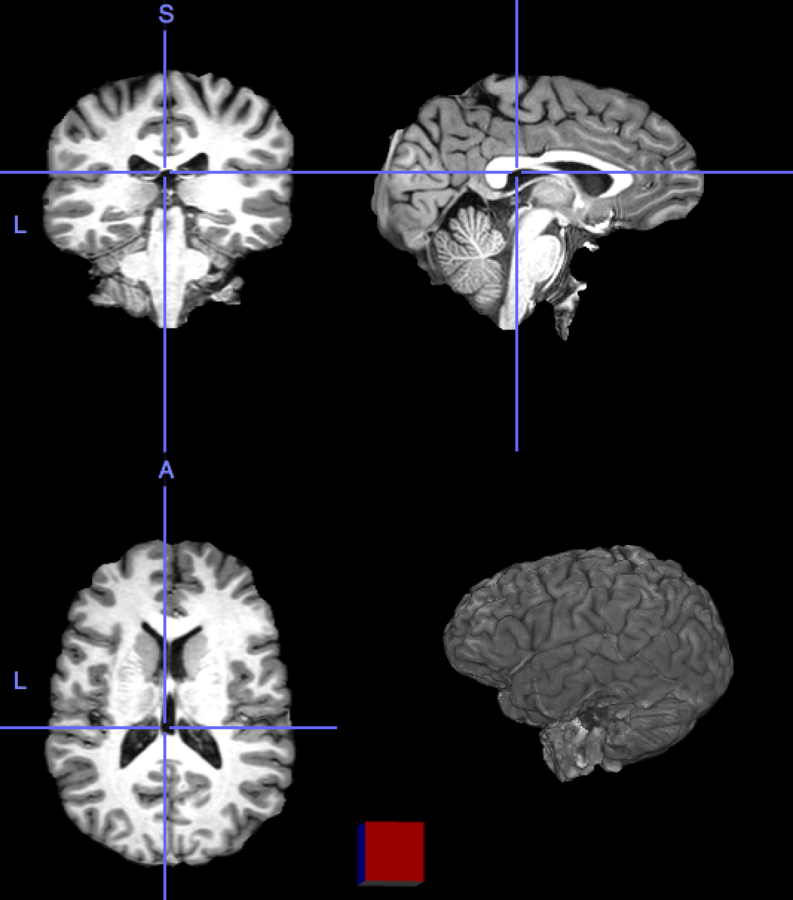
What do you see?
(Almost) any graph-based model is applicable
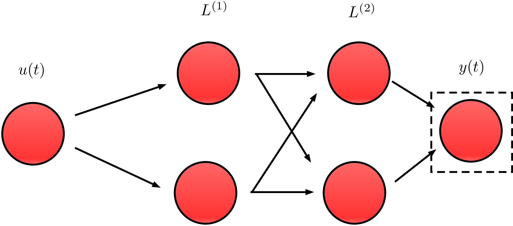
In this work we propose neural networks graphs.
Simplest example: this 2x2 network.
Issue #1: the exponential matrix is heavier to compute as the size of the network grows.
Hence we use the Padé approximation
Theorem:
This condition is true in 2x2 case as
import sympy as s
k11,k12,k21,k22 = s.symbols('k11,k12,k21,k22')
k1,k2,t = s.symbols('k1,k2,t')

A = s.SparseMatrix([[-(k11+k12),0, 0,0],
                    [0,-(k21+k22), 0,0],
                    [k11,k12,      0,0],
                    [k21,k22,      0,0]])

B = s.Matrix([1/3,2/3,0,0])
C = s.Matrix([0,0,k1,k2]).T
Issue #2: A general framework for parameter estimation is needed.
Gradient descent algorithm:
Cost function:

import numpy as np
from scipy impoer convolve1d

def grad_obj(x):
    Ph=[]; Gr=[]
    for i in range(len(x)):
        Ph+=[Phi(x[i])]
        Gr+=[Part(x[i])]

    Gr_est=convolve1d(Gr,u,axis=1).T
    y_est=convolve1d(Ph,u,axis=1).T

    err=y_est-y
    grad_ob=(np.sum(err*Gr,axis=1).T)/err.shape[1]
    return grad_ob
Issue #3: The image size is (182, 218, 182, 23)...
about 7 million voxels per timepoint!
An iterative refinement strategy has been adopted.
Level = 8
Level = 4
Level = 2
Level = 1


4. Results
Hotelling p-value has been calculated for all image pairs in a voxel-wise manner.
A confidence level of 0.05 has been used.
5. Conclusions &
future works
Conclusions:
- A general graph-based framework for PET parameter estimation has been written in Python.
- Voxel-level parameters has showed interesting results in change-detection problem, regardless of the tracer.
Future work:
- Compare the framework's result with commonly-used methods
- Use the framework in other context (e.g. brain tumors)
- Re-write in dask the framework for scalability (parallel/cluster/GPU computing) and computation time reduction
- Test bigger networks
Thank you!
I want to thank for their support:
E. Arbitrio, S. Basso, P. Gallo, E. Perracchione, F. Rinaldi.
References
[1] M. Arioli, B. Codenotti, and C. Fassino, The Padé method for computing the matrix exponential, Linear Algebra and its Applications, 240 (1996), pp. 111–130.
[2] A. Meurer, C. P. Smith, M. Paprocki, et al., SymPy: symbolic computing in Python, PeerJ Computer Science,3 (2017), p. e103.
[3] C. S. Patlak, R. G. Blasberg, and J. D. Fenstermacher, Graphical Evaluation of Blood-to-Brain Transfer Constants from Multiple-Time Uptake Data, Journal of Cerebral Blood Flow & Metabolism, 3 (1983), pp. 1–7.
[4] G. L. Zeng, A. Hernandez, D. J. Kadrmas, and G. T. Gullberg,
Kinetic parameter estimation using a closed-form expression via integration by parts, Physics in medicine and biology, 57 (2012), pp. 5809–21