Cheating with the domain:

the Fake Nodes approach as an interpolation paradigm

Stefano De Marchi, Francesco Marchetti,

Emma Perracchione, Davide Poggiali

D. Poggiali, postDoc

Perugia MATA 2020

Summary:

Intro: What are Fake Nodes?
Relevant Theorems
Numerical Examples
Outro: Future Works

Slides are available online

https://slides.com/davidepoggiali/

1. Intro: What are Fake Nodes?

Interpolation on Fake Nodes, or interpolation via Mapped Bases is a technique that applies to any interpolation method. It has shown in many cases the ability of obtaining a better interpolation without getting new samples.

This means that, provided that the original nodes are a sufficient sample of the given signal, it can be possible in principle to provide an interpolation of smaller error.

1. Intro: what are Fake Nodes?

In terms of code: suppose that you have a generic interpolation function ...

def my_fancy_interpolator(x,y,xx):
  .......
  .......
  return yy

def my_fancy_interpolator(x,y,xx):
  p = np.polyfit(x,y)
  yy = np.polyval(p,xx)
  return yy

for instance ...

instead of calling the function directly you define a mapping function S and interpolate over the fake nodes S(x)

f = lambda x: np.log(x**2+1)
x = np.linspace(-1,1,10)
y = f(x)
xx = np.linspace(-1,1,100)



yy = my_fancy_interpolator(x,y,xx)

f = lambda x: np.log(x**2+1)
x = np.linspace(-1,1,10)
y = f(x)
xx = np.linspace(-1,1,100)

S = lambda x: -np.cos(np.pi * .5 * (x+1))

yy = my_fancy_interpolator(S(x),y,S(xx))

In symbolic terms: given a function

f: \Omega \subseteq \mathbb{R}^d \longrightarrow \mathbb{R}\;\;\;\;\; {d \in \mathbb{N}},

a set of nodes

X = \{ x_0, \dots, x_N \in \Omega \},

and a set of basis functions

\mathcal{B} = \{ b_i: \Omega \longrightarrow \mathbb{R} \}_{i = 0, \ldots, N}

The interpolant is given by a function

\displaystyle \mathcal{P}(\bm{x}) = \sum_{i=0}^{N} c_i b_i(\bm{x})

s.t.

\mathcal{P}(\bm{x}_i)=y_i:=f(\bm{x}_i) \;\;\forall i

\mathcal{B} = \{ b_i \circ S: \Omega \longrightarrow \mathbb{R}^d \}_{i = 0, \ldots, N}

\displaystyle \mathcal{R}^s(\bm{x}) = \sum_{i=0}^{N} c_i b_i(S(\bm{x}))

\mathcal{R}^s(\bm{x}_i)=y_i:=f(\bm{x}_i) \;\;\forall i

This process can be seen equivalently as:

1. An ordinary interpolation over the mapped basis

\[\mathcal{B}^s = \{b_i \circ S \}_{i=0, \dots, N}.\]

[Useful for theorems]

2. An interpolation over the original basis \(\mathcal{B}\) of a function \(g: S(\Omega) \longrightarrow\mathbb{R}\)

on the fake nodes

\[S(X) = \{S(x_i) \}_{i=0, \dots, N}.\]

\(g\in C^s\) must satisfy \(g(S(x_i)) = f(x_i)\;\;\forall i\).

If \(\mathcal{P} \approx g \) on \(S(X)\) with the original basis,

then \(\mathcal{R}^s = \mathcal{P} \circ S \approx f \) on \(X\)

[Useful for computations]

2. Relevant Theorems

Common hypothesis from now on:

(1.) The mapping \(S\) is injective \(\longrightarrow\) Fake Nodes do not overlap

(2.) We interpolate a function \(g\) s.t. \( g\circ S =f\). Such function exists as (1.) holds

Proposition 1. [Equivalence of the Lebesgue constant]

The Lebesgue constant associated to the mapped nodes \(\Lambda^s(\Omega)\) is so that

\[\Lambda^s(\Omega) = \Lambda(S(\Omega)).\]

This means that the interpolation via mapped basis inherits the Lebesgue constant of the original basis in the Fake Nodes.

Lemma 1. [Equivalence of a cardinal basis]

If \(\{u_i\}_{i=0,\dots,N}\) is a cardinal basis on the Fake Nodes \(S(X)\) then

\( \{u_i\circ S\}_{i=0,\dots,N}\) is cardinal too on \(X\)

Proposition 2. [Stability]
Let \(\mathcal{R}^s_{\tilde{f}}\) be the interpolant of the function values

\(\tilde{f}(x_i)\), \(i=1,\ldots,n\). Then,
\[ \lvert\lvert \mathcal{R}_f^s - \mathcal{R}_{\tilde f}^s \rvert\rvert_{\infty,\Omega} \leq \Lambda^s(\Omega) \; \| f-{\tilde f} \|_{\infty, X_n}.\]

This guarantees the stability over (small) perturbation of the interpolant in case the Lebesgue constant at the Fake Nodes is sufficiently small.

Proposition 3. [Error bound inheritance]
The mapped basis interpolation inherits the error bounds of the original bases in any given norm, i.e.
\[\lvert\lvert \mathcal{R}_f^s-f \rvert\rvert_{\Omega} = \lvert\lvert \mathcal{P}_g-g \rvert\rvert_{S(\Omega)}. \]

This theorems links the error bounds. Any error bound found on the interpolation with the original basis \(\mathcal{B}\) on the Fake Nodes \(S(X)\) holds to the mapped basis \(\mathcal{B}^s\) in the original nodes \(X\).

3. Numerical Examples

1). Runge effect (1D)

The Runge effect is taught in every Num. Calculus course. Basically, we avoid it by resampling to Chebyshev or Chebyshev-Lobatto nodes...

...but what if we use a mapping that sends equispaced to CL nodes?

S(x) = - 5\cos(\pi \frac{x+5}{10})

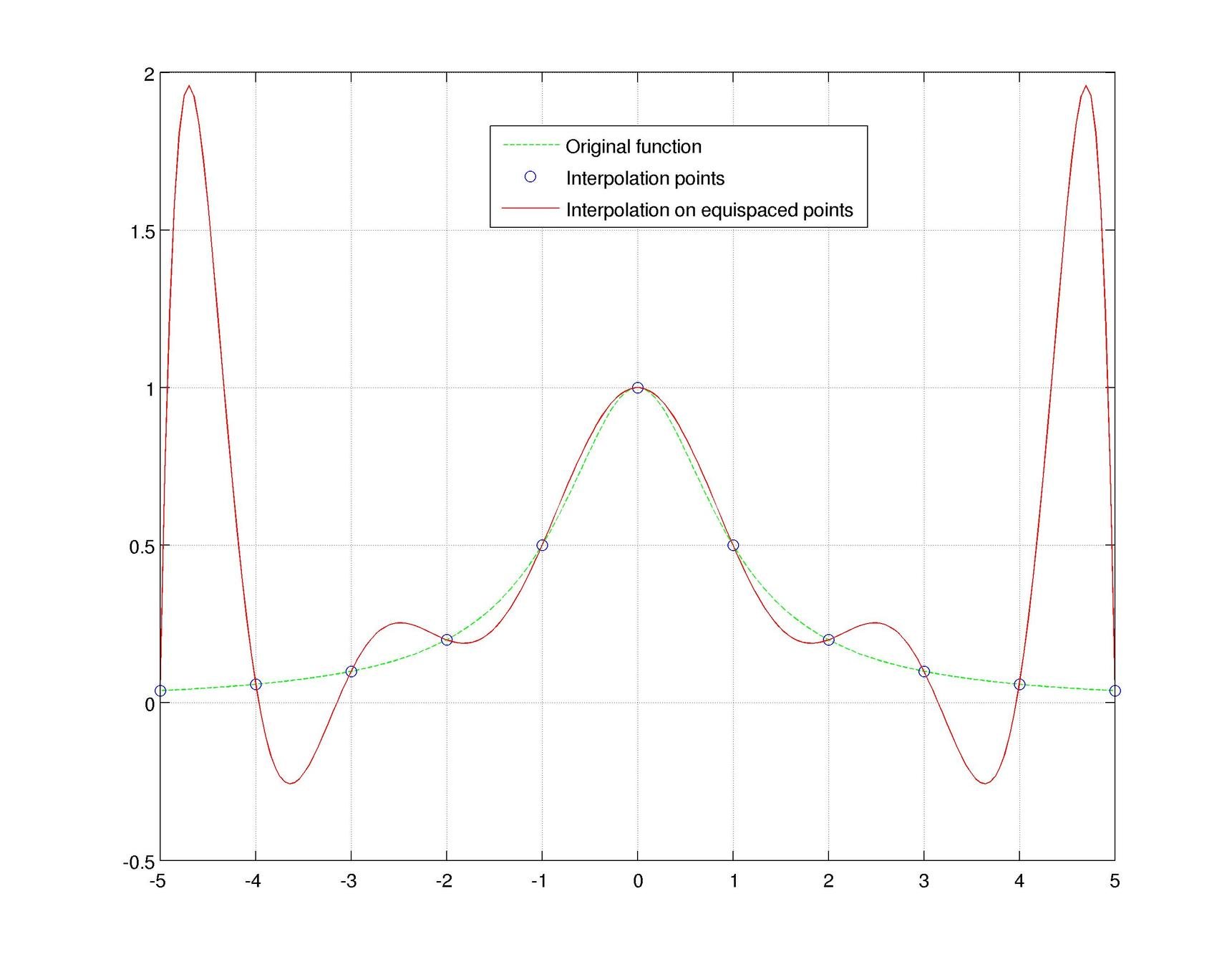
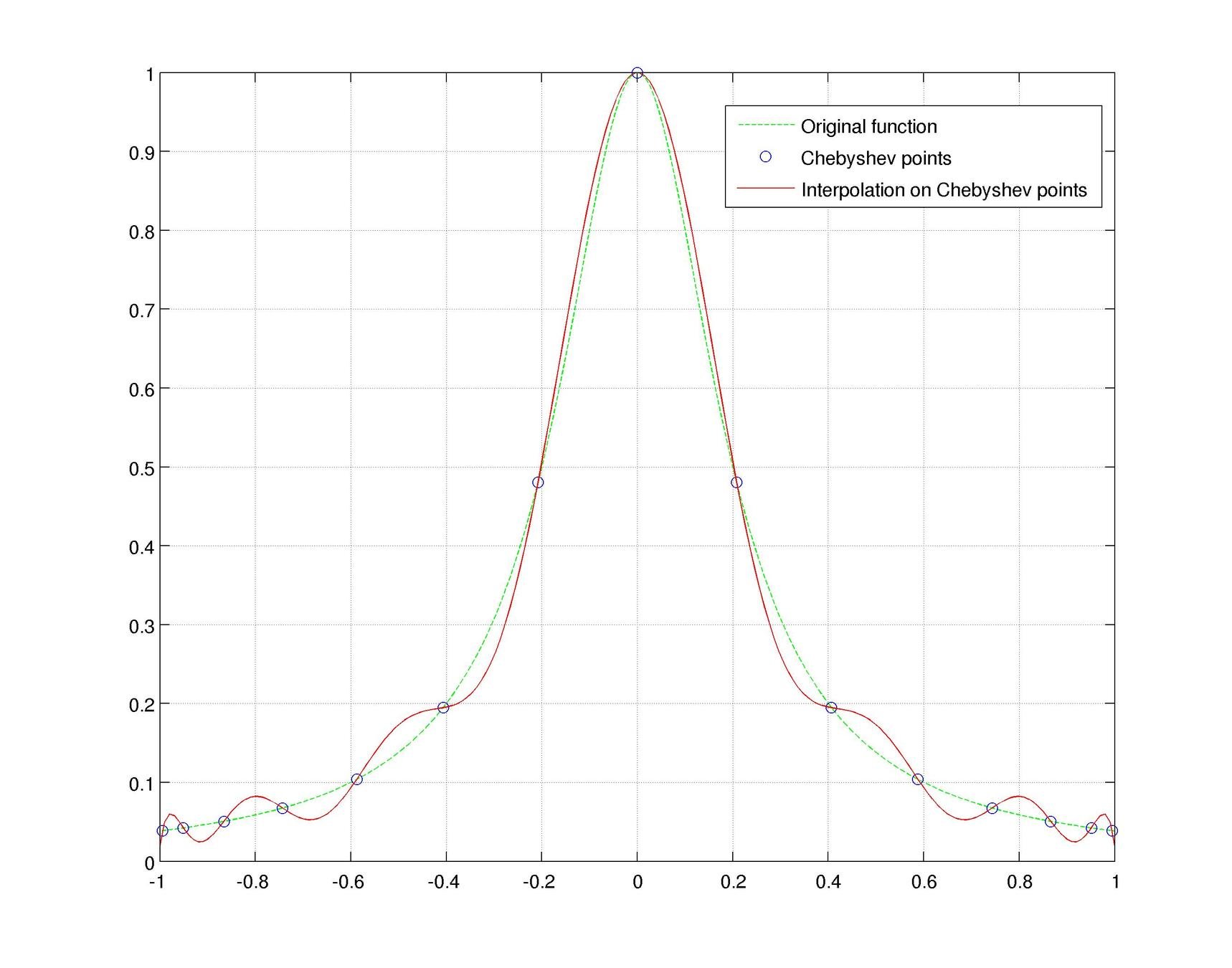
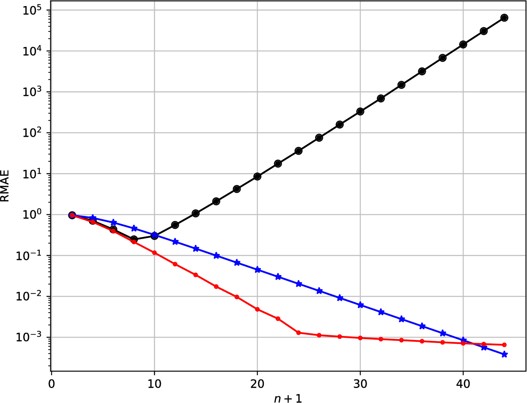
Fake-CL nodes (red) are not always better than actual CL nodes (blue)

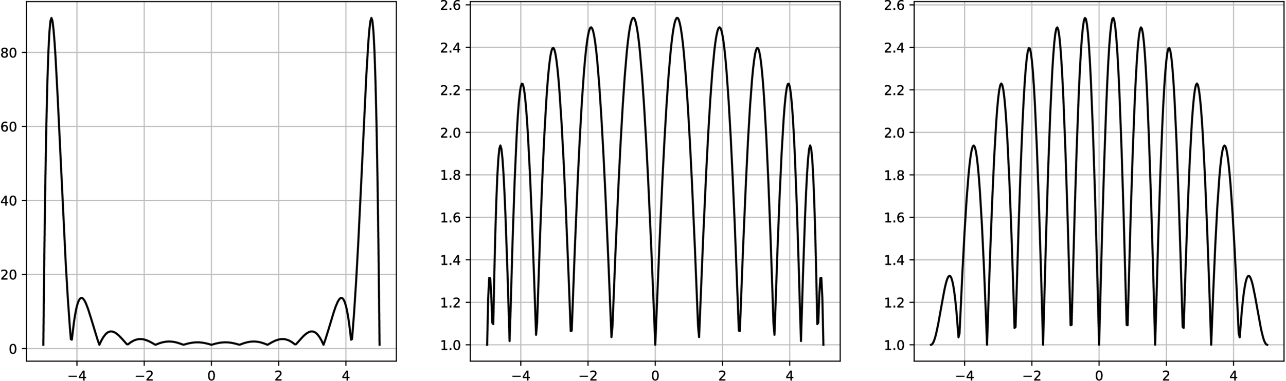
Inheritance of the Lebesgue constant

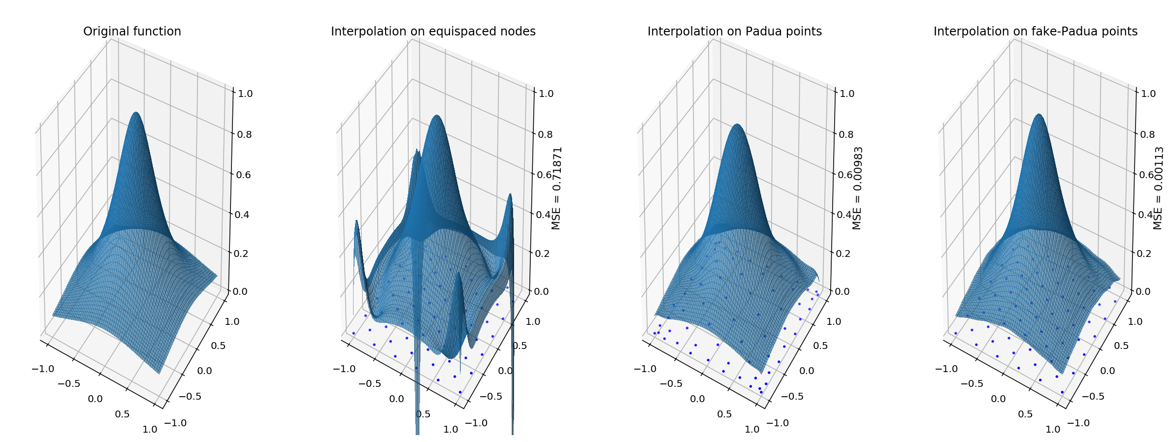
2). Runge effect (2D)

In a similar way we can map a subsampling of the equispaced grid onto the Padua points, with comparable results

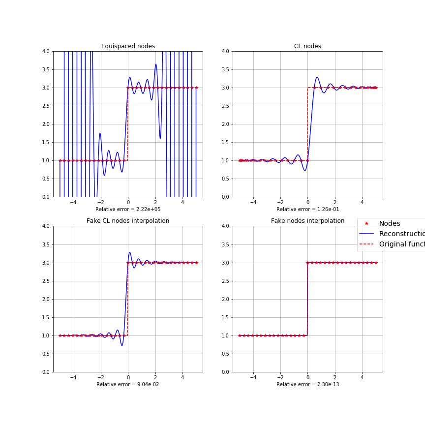
3). Gibbs phenomenon (1D)

If we interpolate a discontinuous function even over CL nodes we observe oscillations around the discontinuity points which grows with the number of samples.

...if we let the polynomial interpolation "breathe" by using a mapping that shift the nodes around all the discontinuity points we can get a good interpolation

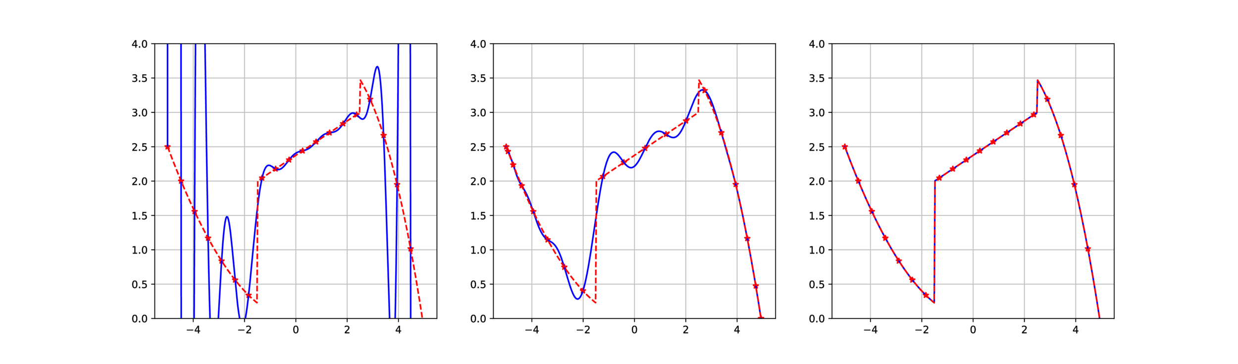
\displaystyle S(x) = x + \sum_{k=1}^m \alpha_k \chi_{\Gamma_k}(x)

\alpha_k \coloneqq k d_k

Same technique, with a more complicated function...

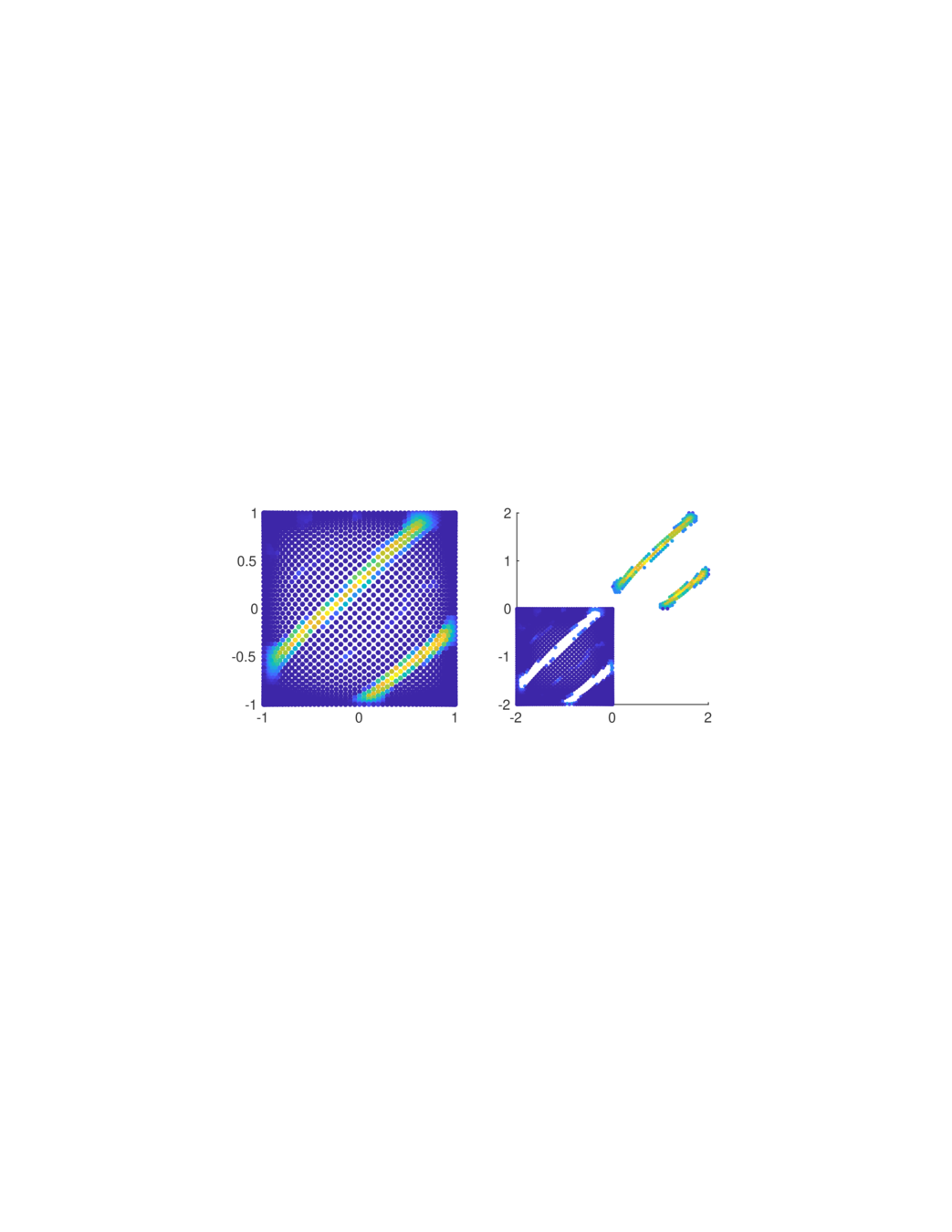
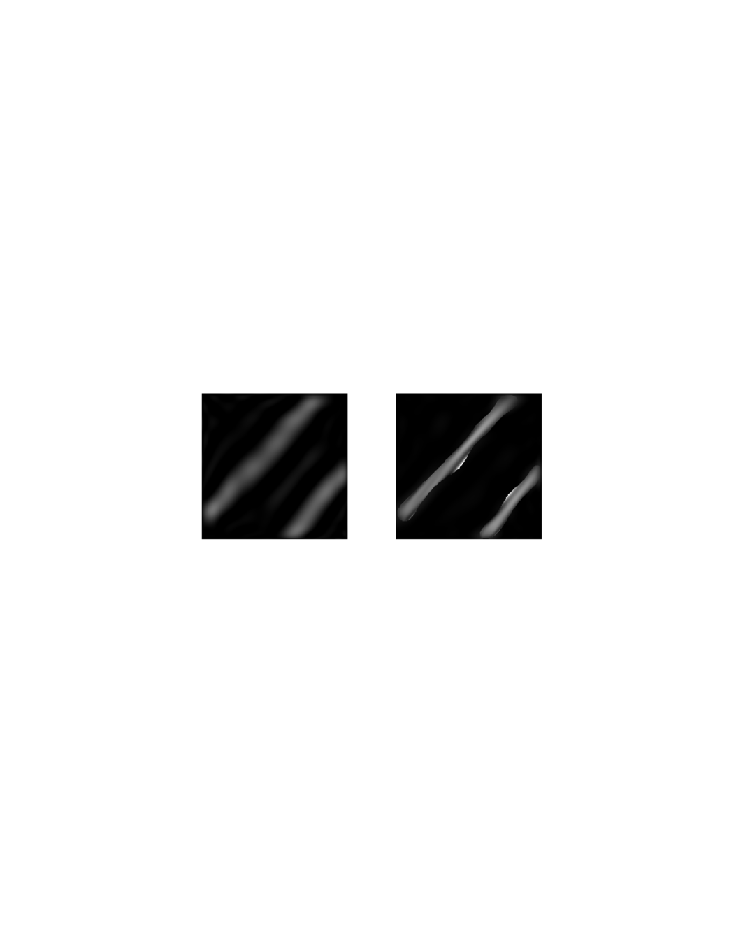
3). Gibbs phenomenon (2D)

A similar mapping function can be used in 2D polynomial approximation.

To recap...

Python code is available online

https://github.com/pog87/FakeNodes

4. Outro: Future Works

Lots of open questions....here are some:

Is there an "optimal" mapping for fixed nodes/FakeNodes couple?
What are the conditions on S to send equispaced nodes onto CL-like nodes?
What is exactly the role of the mapping in error propagation?

Fake RBFs
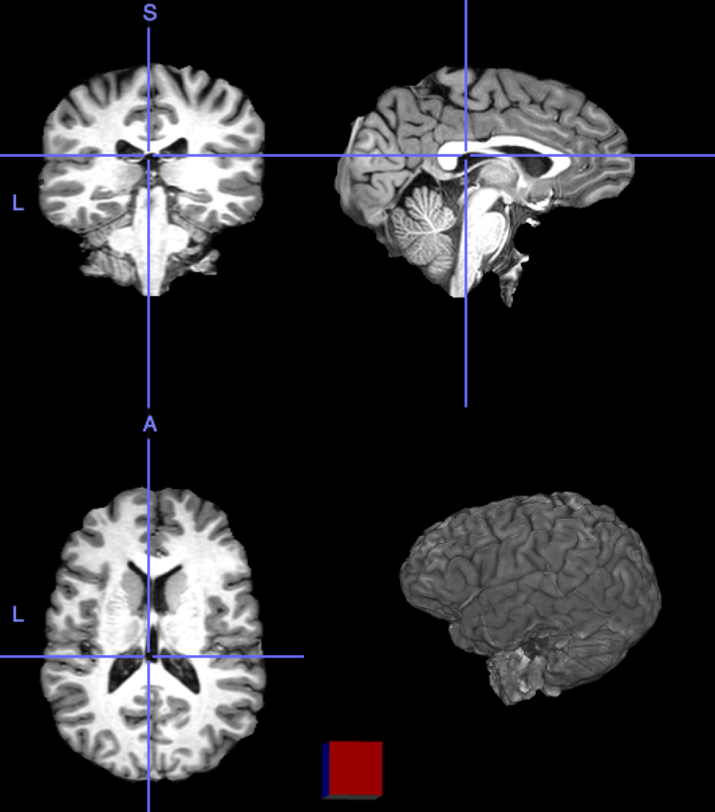
Applications to medical imaging
Least squares approximation
Splines
....

Future works:

References

[1] B. Adcock, R.B. Platte, A mapped polynomial method for high-accuracy approximations on arbitrary grids, SIAM J. Numer. Anal.

[2J P. Berrut, S. De Marchi, G. Elefante, F. Marchetti, Treating the Gibbs phenomenon in barycentric rational interpolation and approximation via the S-Gibbs algorithm. Applied Math. Letters, 2020.

[3] S. De Marchi, F. Marchetti, E. Perracchione, Jumping with Variably Scaled Discontinuous Kernels (VSDKs), BIT Numerical Mathematics 2019.

[4] S. De Marchi, F. Marchetti, E. Perracchione, D. Poggiali, Polynomial interpolation via mapped bases without resampling, JCAM 2020.

[5] S. De Marchi, G. Elefante, E. Perracchione, D. Poggiali, Quadrature at Fake Nodes, preprint 2020.
[6] C. Runge, Uber empirische Funktionen und die Interpolation zwischen aquidistanten Ordinaten, Zeit. Math. Phys, 1901.