Morphological Operators for binary images with applications
Davide Poggiali, University of Padova
Potenza, July 7th 2023
AGRITECH - PNRR
Potenza, July 7th 2023

Davide Poggiali: 36yo
University of Padova
MD Mathematics
PhD Neurosciences

Disclaimers:
- For mathematicians: I tried to keep it simple.
- For non-mathematicians: I really did.

Summary:
- What is a binary image
- Building some morphological operators
- Morphological features calculation
- An example of application
1. What is a binary image
(and where does it come from?)
A greyscale image is a MxN matrix. Its values represent the intensity at the corresponding pixel.
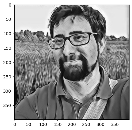
As mathematicians we like to think that the image is a bivariate function sampled over an equispaced grid of nodes.
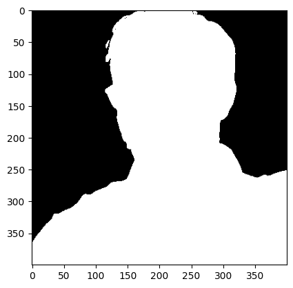
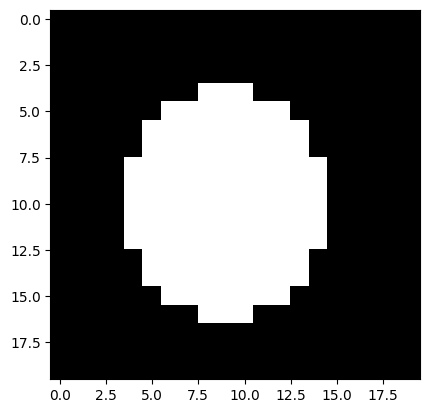
A binary image is a MxN matrix with values in {0,1} where 0 is the background and 1 is the Region Of Interest (ROI).
A binary image can be obtained from a greyscale image by segmentation.
A binary image (n-dimensional) can be represented differently: Let \(I\in \{0,1\}^{N\times\dots \times N}\) be a binary (n-dimensional) image.
\(I\) can be represented as the set of its non-zero indexes,
\(A=\{p| I(p)=1 \}\subset \mathbb{Z}^n .\)
For instance the 2D cross is
\(H=\{(1,0),(0,1),(0,0),(-1,0),(0,-1)\}\)
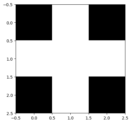
array([[0, 1, 0],
       [1, 1, 1],
       [0, 1, 0]])
2. Building some morphological operators
We can easily define some basic operators on binary images of the form \( A \subset \mathbb{Z}^n\):
- Intersection and union of two images as usual, which corresponds to the voxelwise and/or operations.
- Inversion as the complementary set \(\bar{A}=\{p\notin A\}\)
-
Shift by some vector \(v\in \mathbb{Z}^n\) as the image
\(A_v=\{a+v|i\in A \}\) - Reflection: \(H^* = \{-h | h \in H\}\).
With these basic operators we can define some more complex ones.
Given \(H\in\mathbb{Z}^n\) a structuring element and \(I\) a binary image we can define the following:
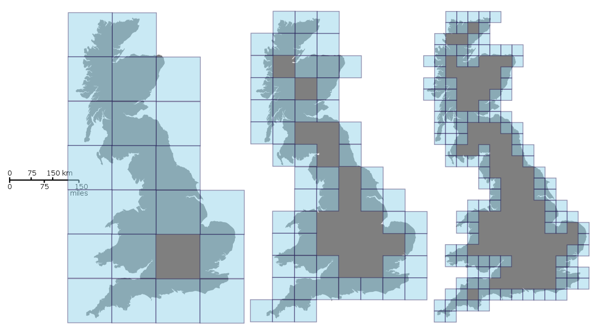
Dilation by \(H\) \[A \oplus H = \{a+h| i \in A, h\in H\}= \bigcup_{h\in H} A_h \]
Erosion by \(H\) \[A \ominus H = \{a-h| i \in A, h\in H\}= \bigcup_{h\in H} A_{-h} \]
Erosion is not the inverse of dilation but
\[A \oplus H = \overline{ \bar{A} \ominus H^*} \]
Let's see some example
With these basic operators we can define some more complex ones.
Given \(H\in\mathbb{Z}^n\) a structuring element and \(I\) a binary image we can define the following:
Opening by H \[I\circ H = (I\ominus H)\oplus H\]
Closing by \(H\) \[I\bullet H = (I\oplus H)\ominus H \]
Let's see some other example
Since it is usual to dilate/erode to get rid of irregularities it is convenient to define:
3. Morphological features calculation
It is useful to extract some features from binary images to quantify their properties.
The first and most simple features are Volume and Surface, than can be calculated with ease in terms of voxels, and converted to absolute measure in case the voxel dimensions are known.
Volume is the easiest to compute as \(Vol(X) = |X|\).
To estimate the surface we can simply measure the border \(\delta X\).
It can be also useful in lots of application to compute the image eccentricity and direction of its main axes.
To compute these features it is necessary to calculate the eigenvalues and eigenvectors of the covariance matrix of the image border.
Another interesting feature to compute is the fractal dimension that describe how much an image is irregularly shaped at its borders.
And finally, we can introduce (but not discuss in detail for timing reasons) some topological features:
- The number of connected components
- The number of holes
- The volume and surface of the convex hull
To compute the error in segmentation we can use the Soreson-Dice coefficient
\[DSC(A,B) = \frac{2 |A \cap B|}{|A| + |B|}\]
as well as the Jaccard Index
\[J(A,B) = {{|A \cap B|}\over{|A \cup B|}} = {{|A \cap B|}\over{|A| + |B| - |A \cap B|}}\]
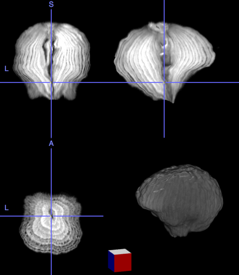
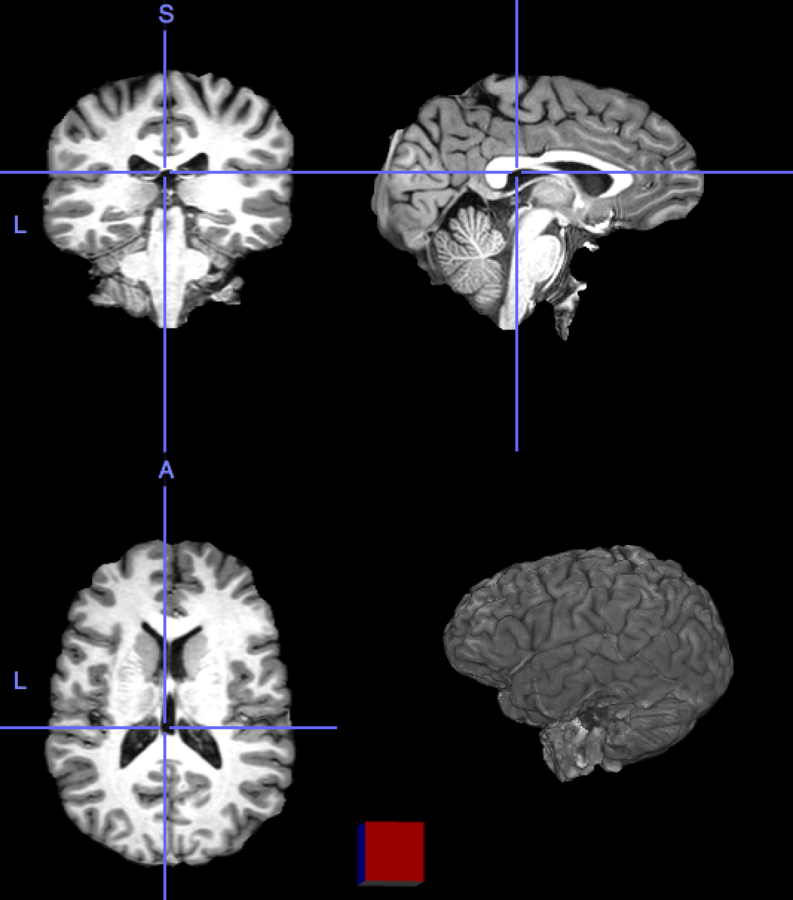
4. An example of application
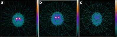
DATscan/Dopa SPECT imaging in PD.
Some open and mathematically interesting problems:
- Calculate the inverse of the dilation/erosion bounded to some features.
- Given an inner ROI and an outer ROI, equally subdivide the space between them.

Essential bibliography:
[1] W. Burger and M. J. Burge, Principles of Digital Image Processing. Springer London, 2009. doi: 10.1007/978-1-84800-195-4.
[2] L. da F. Costa and R. M. Cesar, Jr., Shape Classification and Analysis. CRC Press, 2018. doi: 10.1201/9781315222325.
[3] The Essential Guide to Image Processing. Elsevier, 2009. doi: 10.1016/b978-0-12-374457-9.x0001-7.
[4] A. C. Bovik, Ed., The essential guide to image processing. San Diego, CA: Academic Press, 2009.
Thank you!