


Space-charge distortion of transverse profiles measured by electron-based Ionization Profile Monitors and correction methods based on machine learning
D. Vilsmeier
R. Singh
M. Sapinski
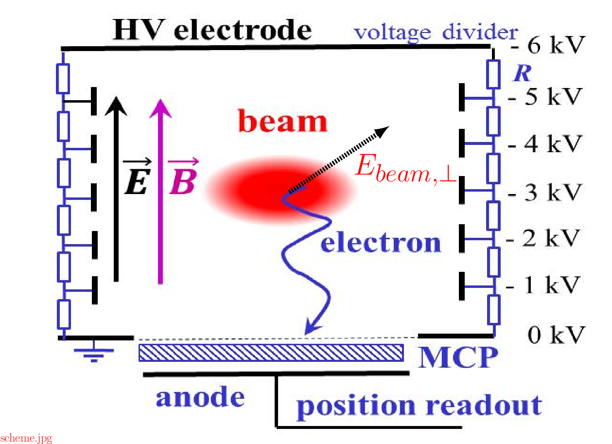
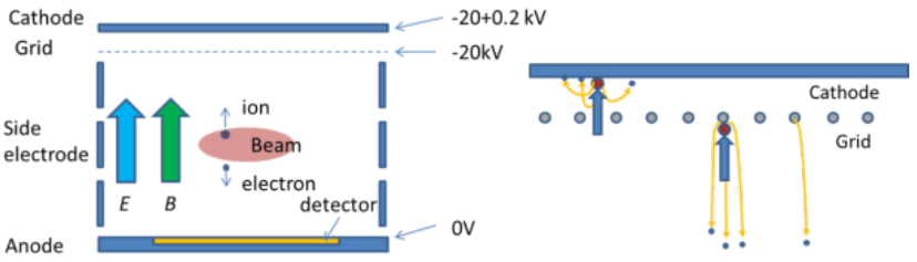
IPM working principle
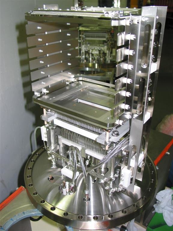
Courtesy of T. Giacomini (GSI)
Courtesy of P. Forck (GSI)
- Rest gas ionization by the beam
- Ionization products (ions/electrons) are transported toward detector
- Non-destructive method
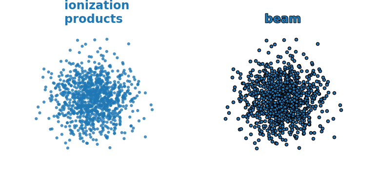
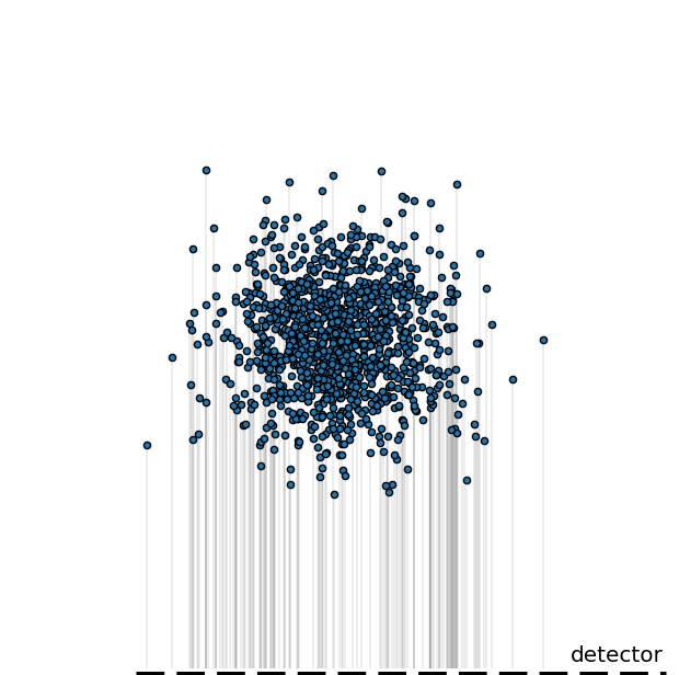
IPM working principle
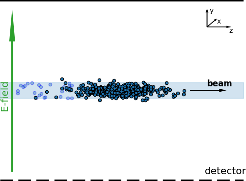
Side view
(beam moves left → right)
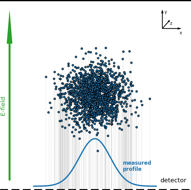
Front view
(beam moves into page)
ionization products
- Measures a projection of the beam profile along one of the transverse dimensions
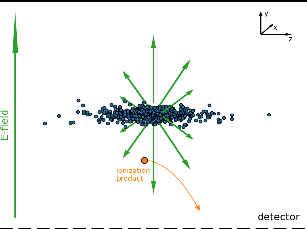
Working assumptions
- The spatial distribution of ionization products follows the transverse beam distribution ✅
- The ionization products don't change their transverse position on the way to the detector ❌
- Detecting ions vs. electrons:
particle mass
momentum transfer obtained from ionization
simplified
✅
❌
Ions vs. electrons
Other benefits of measuring ions:
- Smaller impact of fringe fields from neighboring magnets
-
No background noise from other electron sources
- E.g. from beam losses
- No need for ion-trapping (→ secondary electrons)
→ Electrons, on the other hand, allow for bunch-by-bunch measurement due to smaller extraction times
Interaction with beam fields
Problem: ions/electrons interact with the em-fields of the beam and receive additional momentum and hence displacement
Solution: apply additional magnetic field to confine the motion of ionization products to their gyro-radius
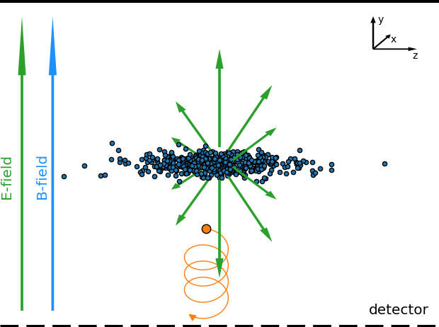
However: magnet needs space & potential corrector magnets & high costs
electrons are quickly removed, i.e. less exposition to beam fields
Profile distortion
Space-charge region
Detector region
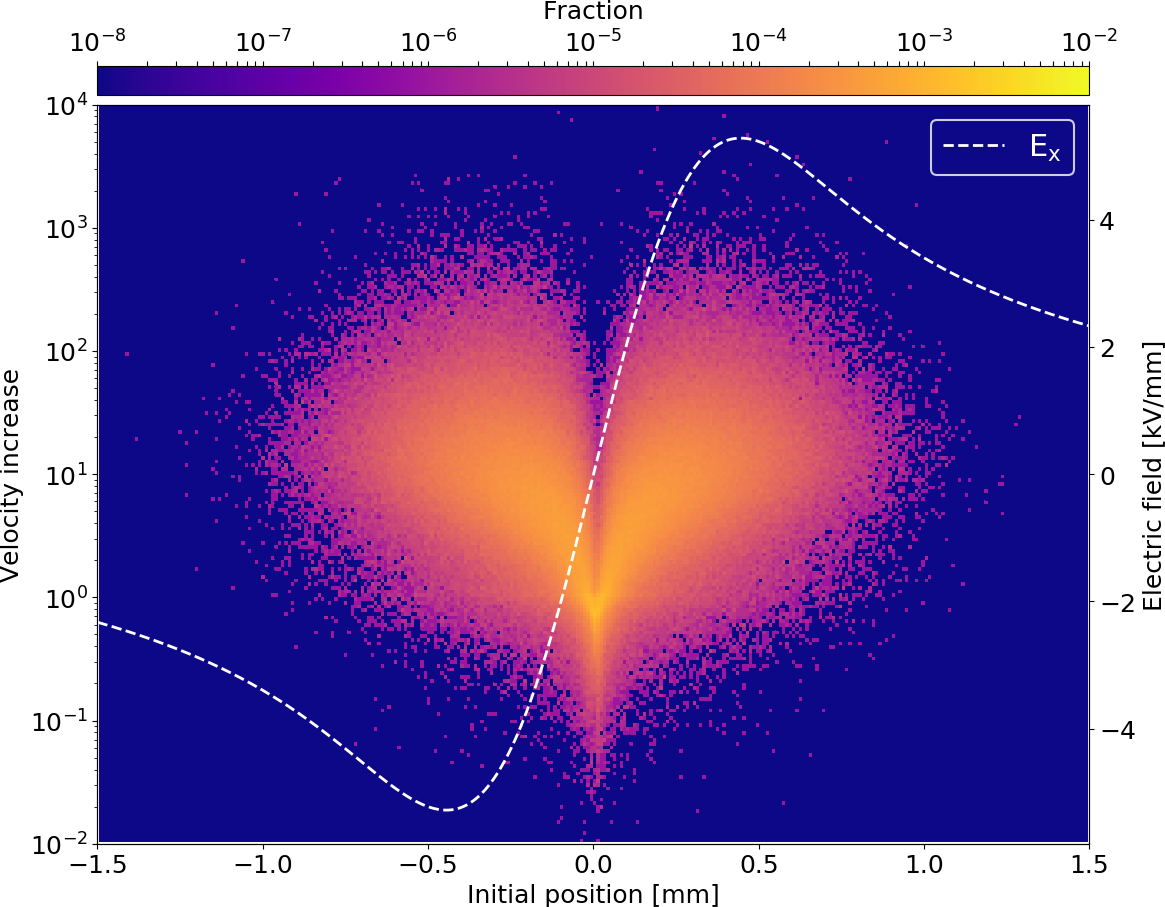
- Complex motion in the external guiding fields (electric + magnetic) as well as beam fields
- Results in significant increase of gyro-radius and thus an increase of potential displacement
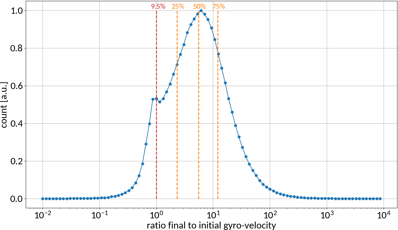
More than 90% of electrons increase their gyro-radius, up to two orders of magnitude
LHC beam
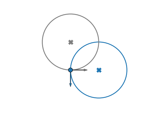
Electron trajectories
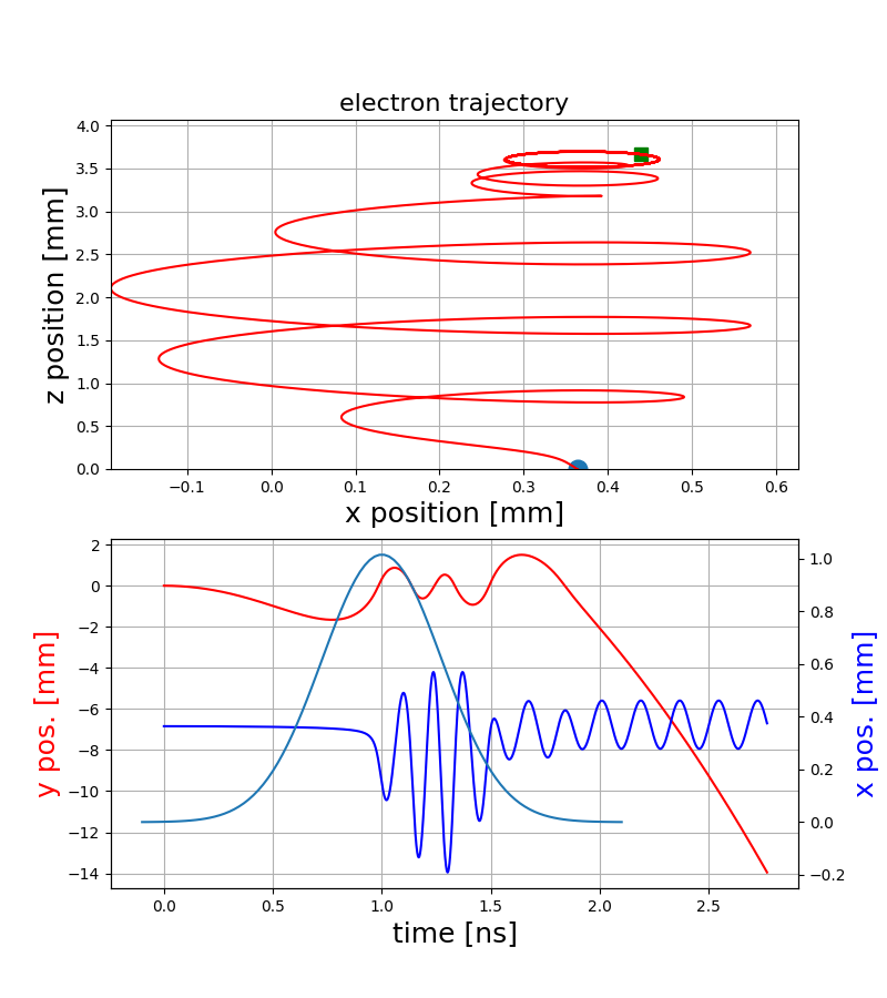
ExB-drift
Polarization drift
Capturing
"Pure" gyro-motion
- The resulting motion strongly depends on the starting position within the bunch and hence on the bunch shape itself
- Various electromagnetic drifts / interactions create a complex dependence of the final gyro-motion on the initial conditions
p-bunch
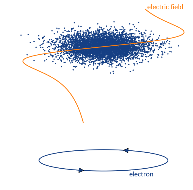
Electron motion
Electron trajectories

Bunch electric field
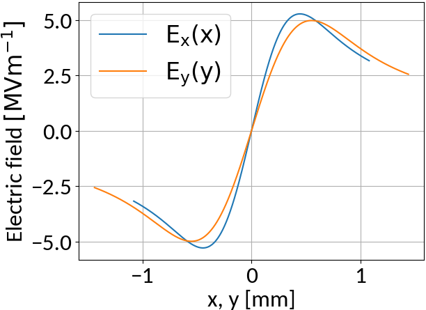
- Depending on the beam parameters, the bunch electric field can become very strong
- Not sufficient to suppress distortion
- Typical values for the electric guiding field are 50 kV/m
Profile distortion

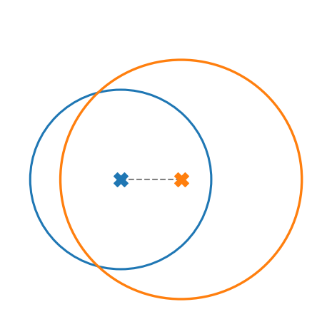
The displacement of measured electrons with respect to their initial position can be split into three distinct contributions:
-
Ionization: displacement of gyro-center due to initial velocity components
-
Space-charge: further shifting of gyro-center
- Gyro-motion: Final position on detector different from the gyro-center
x
z
Profile distortion
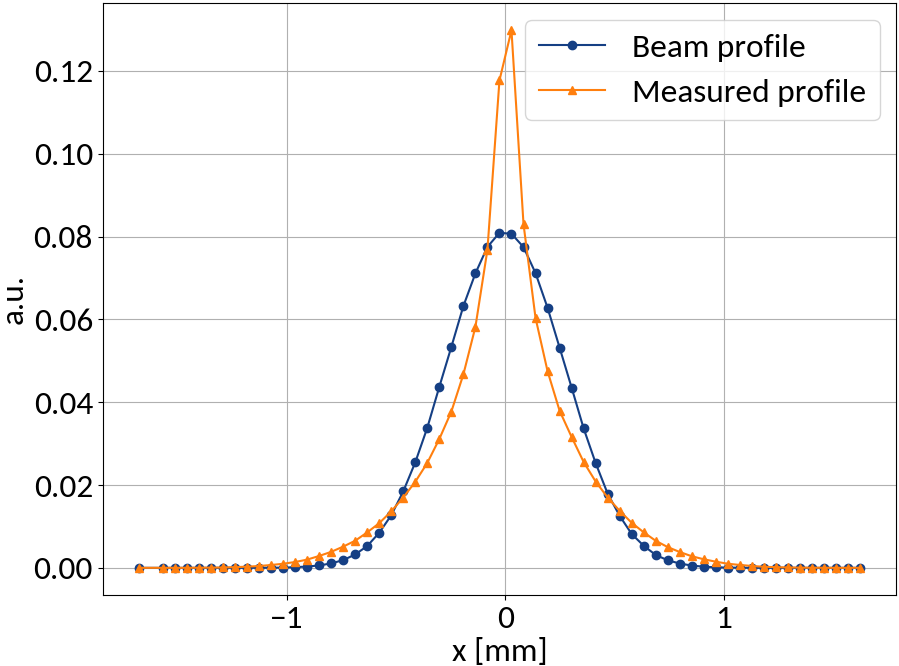
Ideally a one-dimensional projection the the transverse beam profile is measured, but...
LHC
Magnetic field increase
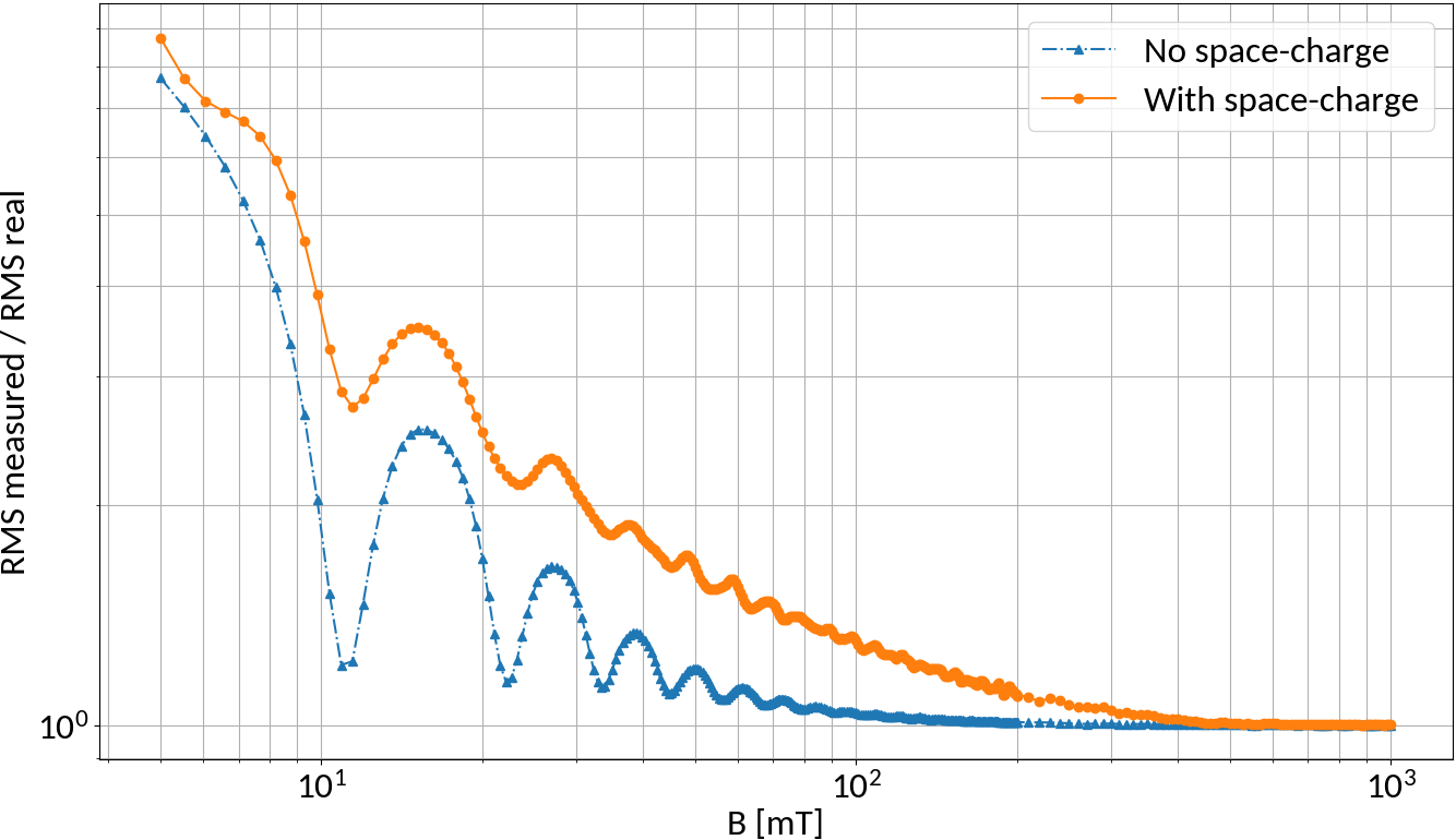
N-turn B-fields
Without space-charge electrons at the bunch center will perform exactly N turns for specific magnetic field strengths
Due to space-charge interaction only large field strengths are effective though
Using Machine Learning
| Parameter | Range | Step size |
|---|---|---|
| Bunch pop. [1e11] | 1.1 -- 2.1 ppb | 0.1 ppb |
| Bunch width (1σ) | 270 -- 370 μm | 5 μm |
| Bunch height (1σ) | 360 -- 600 μm | 20 μm |
| Bunch length (4σ) | 0.9 -- 1.2 ns | 0.05 ns |
Protons
6.5 TeV
4kV / 85mm
0.2 T
Training

Validation

Testing

Used to fit the model; split size ~ 60%.
Check generalization to unseen data; split size ~ 20%.
Evaluate final model performance; split size ~ 20%.
Consider 21,021 different cases
1
2
3
🠖 Evaluated on grid data and randomly sampled data

Generate training data via simulation
Virtual-IPM simulation tool was used to generate the data
| Parameter | Range | Step size |
|---|---|---|
| Bunch pop. [1e11] | 1.1 -- 2.1 ppb | 0.1 ppb |
| Bunch width (1σ) | 270 -- 370 μm | 5 μm |
| Bunch height (1σ) | 360 -- 600 μm | 20 μm |
| Bunch length (4σ) | 0.9 -- 1.2 ns | 0.05 ns |
Protons
6.5 TeV
4kV / 85mm
0.2 T
= 21,021 cases | 5h / case | 12 yrs | Good thing we have computing clusters :-)
(1)
(1) Virtual-IPM is not limited to IPM simulations, it supports a wide range of applications including BIF, gas jet, etc.
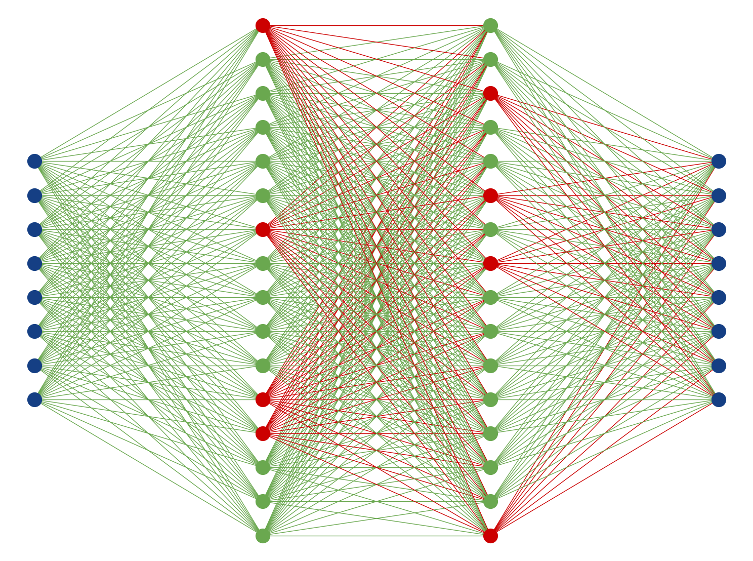
Artificial Neural Networks
Input layer
Weights
Bias
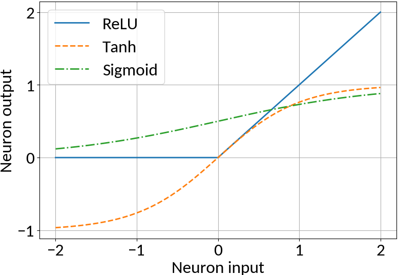
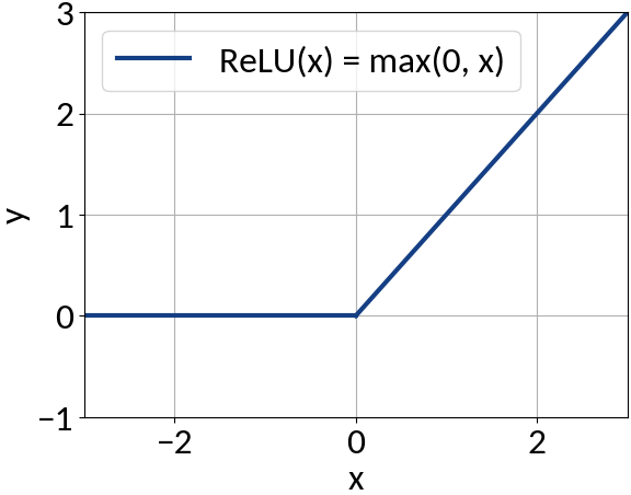
Apply non-linearity, e.g. ReLU, Tanh, Sigmoid
Perceptron
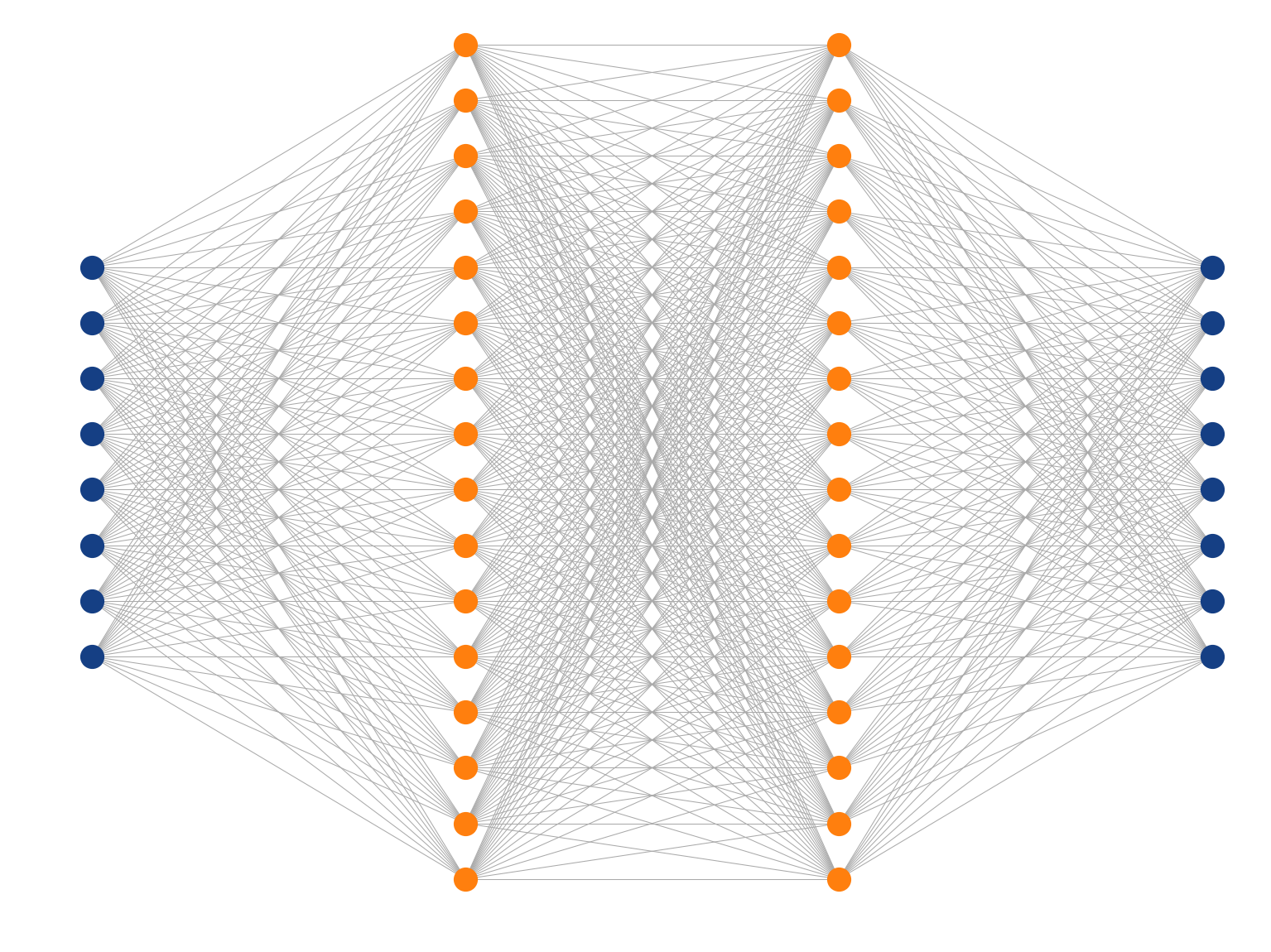
Multi-Layer Perceptron
Inspired by the human brain, many "neurons" linked together
Map non-linearities through non-linear activation functions
ANN Implementation
IDense = partial(Dense, kernel_initializer=VarianceScaling())

# Create feed-forward network.
model = Sequential()

# Since this is the first hidden layer we also need to specify
# the shape of the input data (49 predictors).
model.add(IDense(200, activation='relu', input_shape=(49,))
model.add(IDense(170, activation='relu'))
model.add(IDense(140, activation='relu'))
model.add(IDense(110, activation='relu'))

# The network's output (beam sigma). This uses linear activation.
model.add(IDense(1))
model.compile(
optimizer=Adam(lr=0.001),
loss='mean_squared_error',
)
model.fit(
x_train, y_train,
batch_size=8, epochs=100, shuffle=True,
validation_data=(x_val, y_val),
)
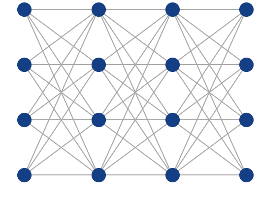
Fully-connected
feed-forward
network
with ReLU
activation
function
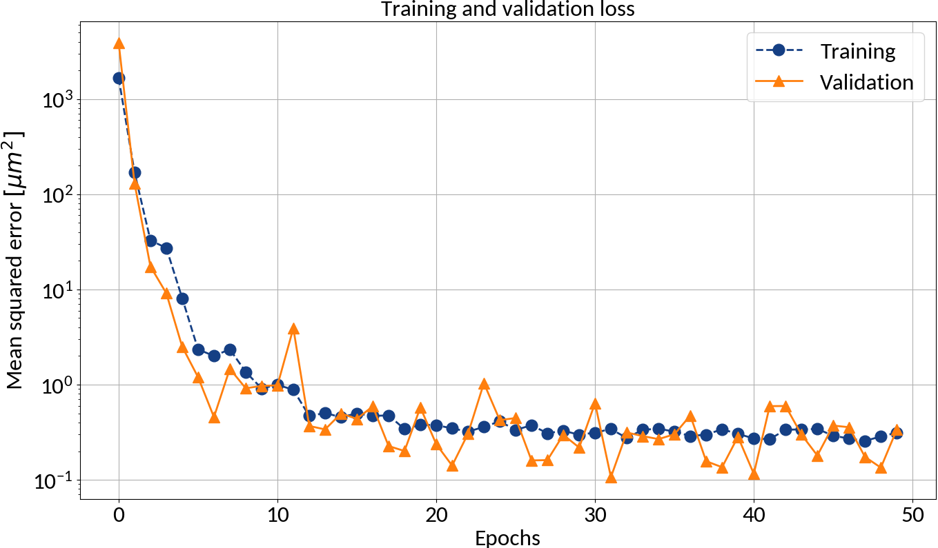
After each epoch compute loss on validation data in order to prevent "overfitting"
Batch learning
🠖 Iterate through training set multiple times (= epochs)
🠖 Weight updates are performed in batches (of training samples)
keras
keras
Profile RMS Inference - Results
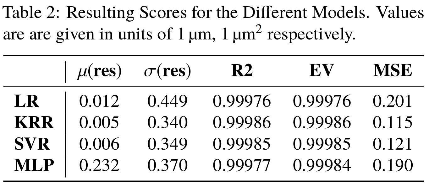
Tested also other machine learning algorithms:
• Linear regression (LR)
• Kernel ridge regression (KRR)
• Support vector machine (SVR)
Multi-layer perceptron (= ANN)
Very good results on simulation data 🠖 below 1% accuracy
Results are without consideration of noise on profile data
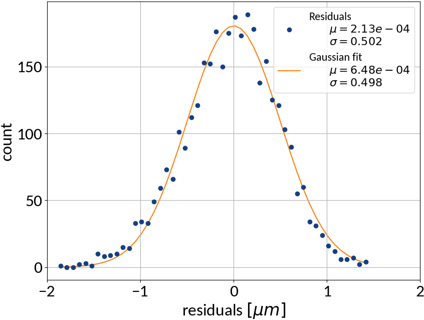
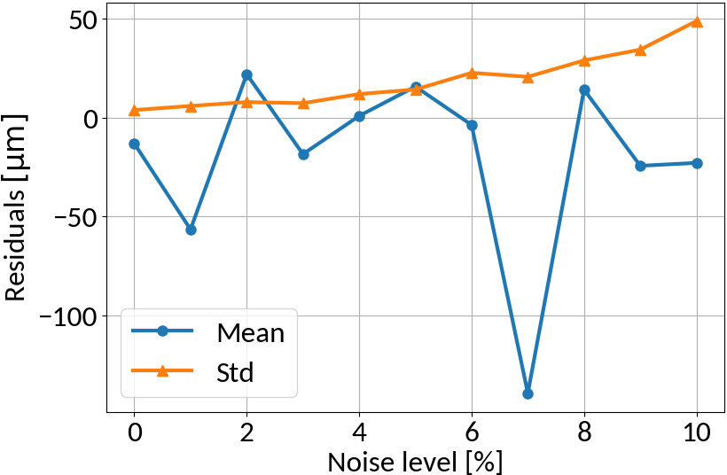
RMS Inference with Noise
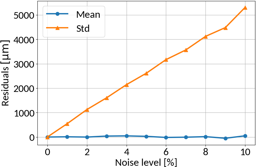
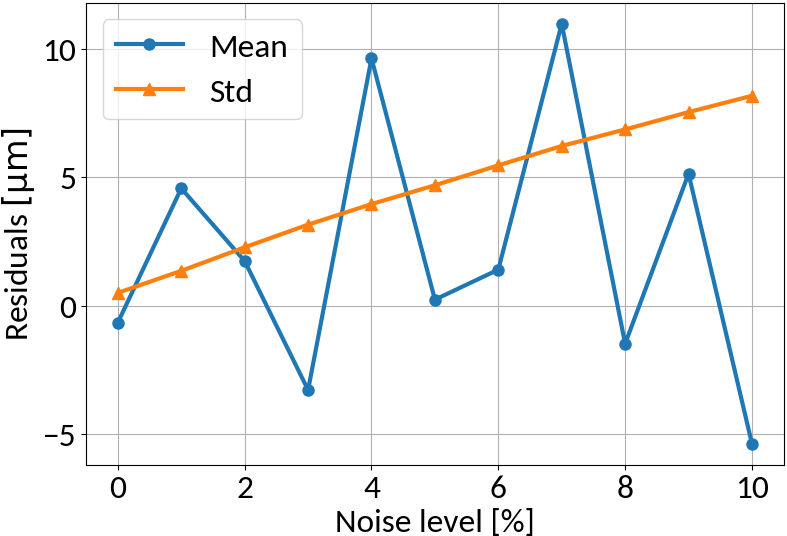
Linear regression model
no noise on training data
similar noise on training data
Linear regression amplifies noise in predictions if not explicitly trained
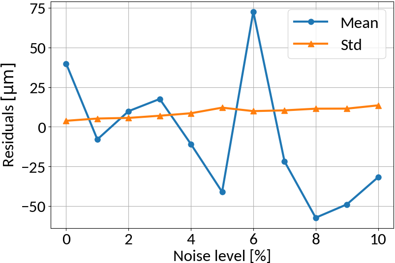
Multi-layer perceptron
MLP amplifies noise; bounded activation functions could help; as well as duplicating data before "noising"
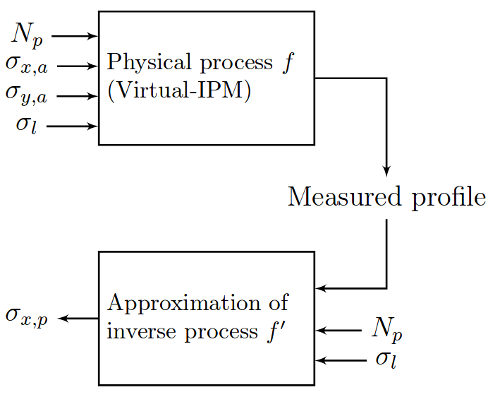
Full Profile Reconstruction
So far:
Machine Learning Model
Instead:
Machine Learning Model
Compute beam RMS
Compute beam profile
Profile distortion: Revisited
-
Divide the x-dimension into several discrete bins; these bins correspond to the detector elements (e.g. wires or pixels of a camera)
- The measured distorted profile emerges as a collection of electrons, each starting at some bin j and being detected at (another) bin i
transformation matrix; represents the probability that an electron which was created at position j is collected at position i;
→ depends on beam parameters / beam distribution
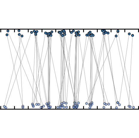
Assumption: no electrons are being lost in the process
i
j
i
j
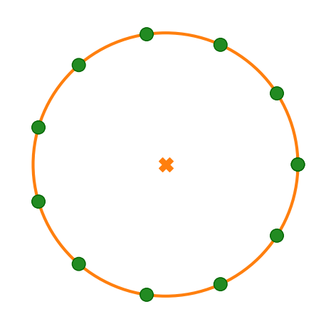
Displacement from gyro-motion
Provided that the moment of detection is random, the gyromotion of electrons gives rise to probabilities of being detected at a specific position.
Applying the limit results in divergence at the "edges" of the motion, so the expression is only valid for the center. For real profiles however we can work with a discretized version of the abovementioned relation.
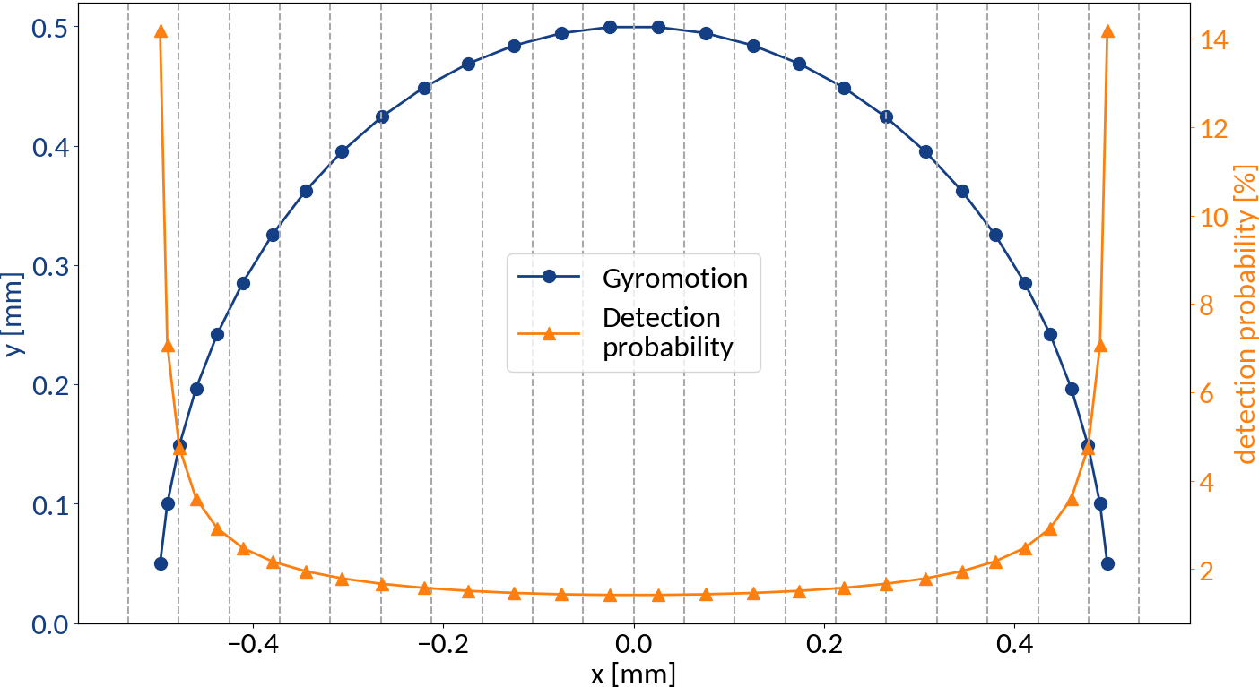
Displacement from gyro-motion
Gyro-radius increase is non-uniform along the original beam profile
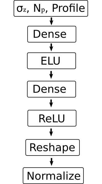
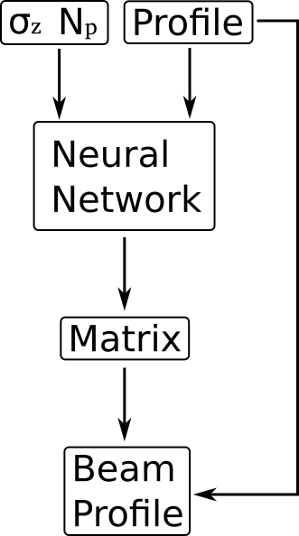
Full profile reconstruction via ANN
Main task of the ANN is to generate the inverse of the transformation matrix:
Together with the original profile, the reconstructed profile can be obtained
The final multiplication must be part of the ANN in order for the backpropagation to work; i.e. no simple feed-forward architecture
Full profile reconstruction via ANN
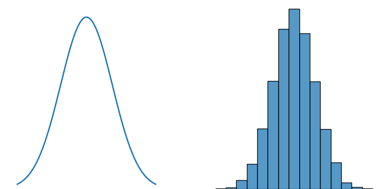
Also attempted "classical" feed-forward architecture, however the results strongly depended on the applied data transformation for the profiles:
- Profiles are given as histograms with arbitrary intensity
- Natural way to normalize would be to divide by the integral, however the network could not be fitted that way
- Only worked for per-feature normalization (center + variance-scale)
- Generalization to non-Gaussian shapes could only be achieved for small deviations
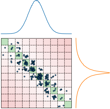
The matrix-generator network from the previous slide works with per-sample normalization

D
a
t
a
s
e
t
row-wise,
per sample normalization
column-wise,
per feature normalization
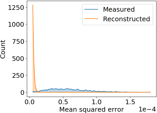
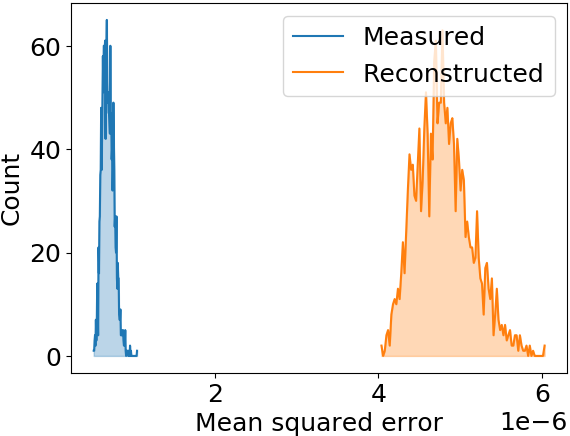
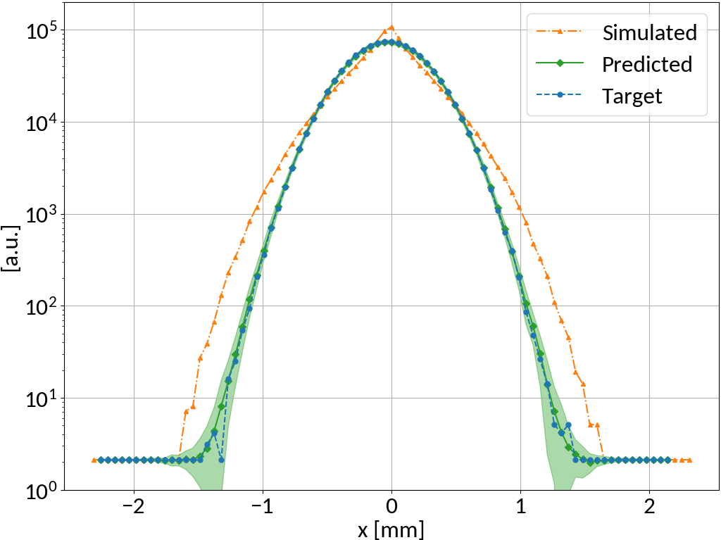
Full profile reconstruction - Results
Performance measure
- Mean squared error (MSE)
prediction
target
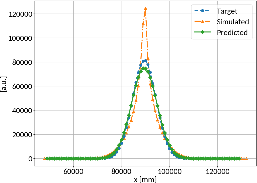
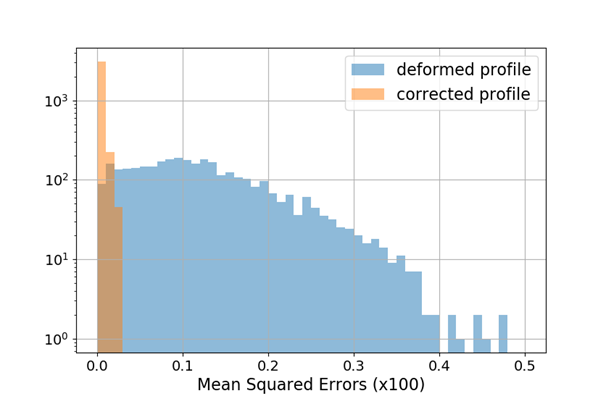
Mean squared error is effectively reduced, profile shape is restored as well
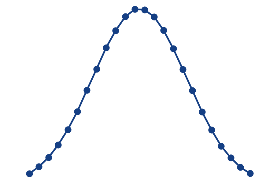
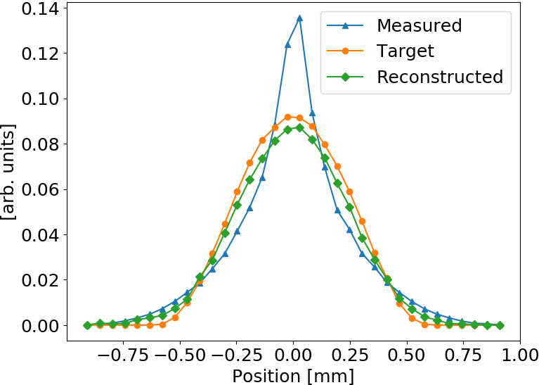
Test: Generalized Gaussian shape
Gen. Gaussian used for testing while training (fitting) was performed with Gaussian bunch shape

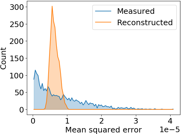
Smaller distortion in this case
ANN model generalizes to different beam shapes
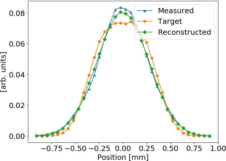
Max. MSE examples
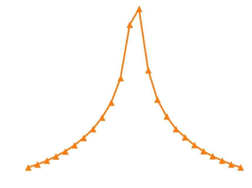
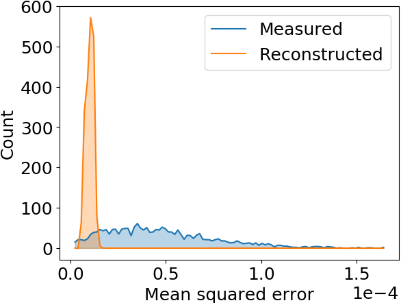
Test: Q-Gaussian shape
Q-Gauss used for testing while training (fitting) was performed with Gaussian bunch shape
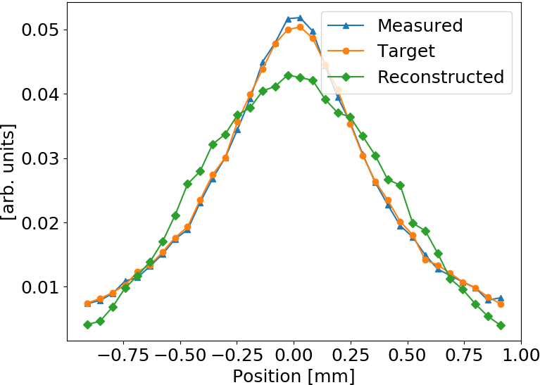
These profiles are significantly wider than the ones used during training
ANN model generalizes to different beam shapes
Model prediction uncertainty
- Could train multiple models with different initialization and different data presentation 🠖 ensemble of predictions
- Emulate multi-model ensemble by using Dropout layers (also for predictions)
inactive
active
ANN shows very small standard deviation in predictions 🠖 the fitting converged well, small model uncertainty
Other possibility: Snapshot Ensembles
Sub-resolution measurements
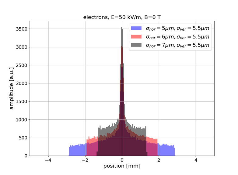
- Understanding or (machine) "learning" beam profile deformation (and how to revert it), this information could be used to measure beams that are smaller than the resolution of the detector (by provoking a deformation / blow-up, then reverting it)
- Example: SwissXFEL, 5.8 GeV electrons, 230 pC bunch charge, 21 fs bunch length, 5-7 μm transverse size
- Beam size is 1/10-th of detector resolution however the deformed profile is well above and strongly depends on the beam size
- Alternative to R. Tarkeshian et al. Phys. Rev. X 8, 021039 (reconstruction based on ion energies)
preliminary
Summary
- Successful beam RMS reconstruction with various machine learning models
-
Reconstruction of complete profiles with artificial neural network:
- The mapping generalizes to different beam shapes
- Model seems to "learn" the distortion mechanisms rather than specific beam shapes
- These methods could potentially be used to measure sub-resolution beam profiles
Outlook
- Verification of feasibility with experimental data (ongoing)
- Comparison with ground truth data obtained from another beam profiler (e.g. OTR)
Literature
- D. Vilsmeier, M. Sapinski, and R. Singh, Space-charge distortion of transverse profiles measured by electron-based ionization profile monitors and correction methods, Phys. Rev. Accel. Beams 22, 052801, 2019
- M. Sapinski, R. Singh, J.W. Storey and D.M. Vilsmeier, Application of Machine Learning for the IPM-Based Profile Reconstruction, Proc. 61st ICFA Advanced Beam Dynamics Workshop (HB'18), Daejeon, Korea, 17-22 June 2018
- D. Vilsmeier, M. Sapinski, R. Singh and J.W. Storey, Reconstructing space-charge distorted IPM profiles with machine learning algorithms, J. Phys.: Conf. Ser. 1067 072003, 2018
- R. Singh, M. Sapinski and D.M. Vilsmeier, Simulation Supported Profile Reconstruction With Machine Learning, Proc. of International Beam Instrumentation Conference (IBIC'17), Grand Rapids, MI, USA, 20-24 August 2017
- ... and references contained therein.