Master Data Science - 2017/2018
Online Learning - Prof. Pierre ALQUIER
On Bayesian UCB for Bandit Problems
Firas JARBOUI
Imad EL HANAFI
Table of contents
- Setting and presentation of the problem
- Frequentist setting
- Bayesian setting
- Optimal policies
- Lai & Robins Lower bound
- UCB Based algorithms
- Frequentist UCB
- Bayesian UCB
- KL-UCB
- Framework
- Numerical results
Settings
- K arms with distributions
$$\nu_{\theta_j}$$
- Multi-Armed-Bandits
- Drawing arm j results in a reward
$$X_t = Y_{t,j}$$
- At each time step t, an agent choose an arm according to a strategy (sampling policy)
$$ (I_t)_{t \geq 0}$$
- Arms are supposed independent
- Goal : maximize the expected cumulative reward until time n
$$ \mathbb{E}(\sum_{ i = 1}^{n}{X_t})$$
Frequentist Bandits
-
$$ \theta_1 ... \theta_K $$
are unknown parameters
-
$$Y_{t,j}$$
iid with distribution
$$\nu_{\theta_j}$$
and mean
$$\mu_{j}$$
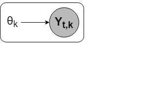
- Maximize the expected cumulative reward is equivalent to minimize the cumulative regret
$$ R_n(\theta) = \mathbb{E}_\theta(\sum_{ i = 1}^{n}{\mu^* - \mu_{I_t}})$$
Bayesian Bandits
-
$$ \theta_1 ... \theta_K $$
are drawn from a distribution
-
$$Y_{t,j}$$
iid with distribution
$$\nu_{\theta_j}$$
$$(\pi_j)_{1 \leq j \leq K}$$
- Maximize the expected cumulative reward
$$\mathbb{E}(\sum_{ i = 1}^{n}{X_i})$$
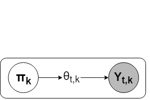
❗️
Expectation is taken over the entire probabilistic model, including the randomisation over
- Equivalent to minimize the Bayes regret
$$ \theta $$
$$R_n^B=\mathbb{E}(R_n(\theta)) = \int R_n(\theta)d \pi (\theta)$$
The paper approach
Aim of the paper :
Show that the Bayesian agent (UCB-Bayes) performs well (compared to UCB) when applied in a frequentist perspective.


Optimal Policies - Lower bound
- Lai & Robbins provided a lower bound for strategy having o(n) regret for all bandit problems.
- For any arm j such that
$$ \mu_j < \mu^* $$
- Regret can be seen written as
$$R_n(\theta) = \sum_{j = 1}^{K}{(\mu^* - \mu_j) \mathbb{E}_\theta(N_n(j))} $$
Where Nn(j) is the number of draws of arm j up to time n
$$ \lim_{n\to\infty} inf \frac{\mathbb{E}_\theta N_n(j)}{log(n)} \geq \frac{1}{inf_{\theta \in \Theta : \mu(\theta) > \mu^*} KL(\nu_{\theta_j}, \nu_{\theta})}$$
UCB based algorithm
- For each arm a, build a confidence interval on µa
- Theoretical result : For every α>2 and every sub-optimal arm, there exist Cα > 0 such that
- Action at time t+1
$$I_{t+1} = argmax_a UCB_a(t) $$
$$UCB_a(t) = \hat{\mu (t)} + \sqrt{\alpha log(t) /2N_a(t) }$$
$$ \mathbb{E}_{\theta}N_T(a) \leq \frac{2\alpha}{\mu^* - \mu_a}log(T) + C_{\alpha} $$
Bayesian Algorithm
$$ \theta_1 ... \theta_K $$
are drawn from a distribution
$$Y_{t,j}$$
iid with distribution
$$\nu_{\theta_j}$$
$$(\pi_j)_{1 \leq j \leq K}$$
-
-
-
To define the bayesian strategy, we start from an initial
prior
$$(\pi_j^0)_{1 \leq j \leq K}$$
Due to independent choice of ϴ, after t round is approximated by the posterior distribution (from agent point of view):
$$ \pi_j^t(\theta_j) \propto \nu_{\theta_j}(X_t) \pi_{j}^{t-1}(\theta_j) $$
$$\text{if}\ I_t = j\ \text{and reward is }\ X_t = Y_{t,j}$$
$$ \pi_i^t = \pi_i^{t-1}$$
$$\text{if}\ i\neq j $$
$$(\pi_j)_{1 \leq j \leq K}$$
UCB-Bayesian Algorithm
- Inspired from Bayesian modeling of the bandit problem
- The agent builds a belief on the distribution of parameters and update it at each iteration.
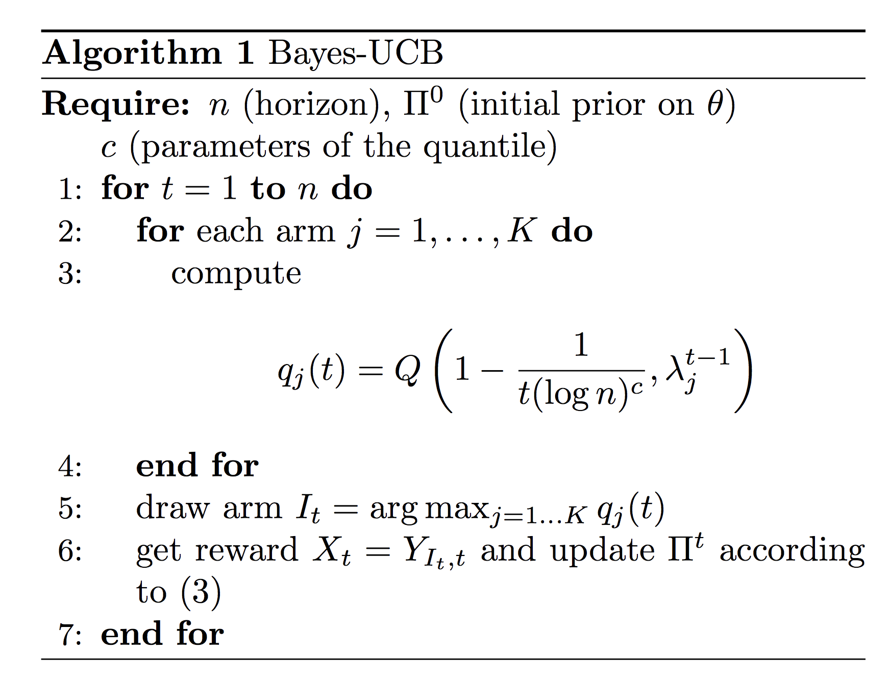

Theoretical performances of Bayes-UCB
- For each arm j compute the quantile of the prior
distribution over the expected reward
- Theoretical result for binary rewards : $$ \text{for any } \epsilon > 0 \text{ and given } c = 5$$
We have the following bound over the expectation of drawing a sub-optimal arm
- Action at time t+1
$$I_{t+1} = argmax_j q_j^t $$
$$q_j^t = Q(1 - \frac{1}{t.log(t)^c},\lambda_j^t)$$
$$ \mathbb{E}_{\theta}N_T(a) \leq \frac{1+\epsilon}{d(\mu^* ,\mu_a)}log(T) + o(log(T)) $$
$$ 1 - \frac{1}{t.log(t)^{c}} $$
Choice of the prior for Bayesian UCB
Non informative prior for the UCB Bayes
- Reduce convergence speed
- Avoid bias in the posterior distribution
Prior that carry useful information for the inference (within the same conjugate family)
- Quantiles are easy to compute (closed form)
- Enhance convergence speed
- Can induce bias
- Allow solving sparsity issues in linear bandit problems
KL-UCB
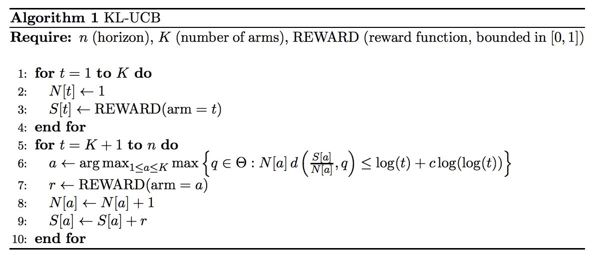
- A UCB-like algorithm
- Upper bound is computed with respect to the distribution (KL-distance)
- In the special case of Bernoulli rewards, it reaches the lower bound of Lai and Robbins
Framework

Object class: Arm
- Generate rewards given
- Characterized for each given setting

Object class: Agent
- Generate Decisions
- Update Information under a reward and a decision
- Characterized for each given setting
Object Class : Simulation
- Takes an Agent and Arm objects
- Simulates the output
Numerical Results
Frequentist setting - Bernoulli - .1 vs .2 -
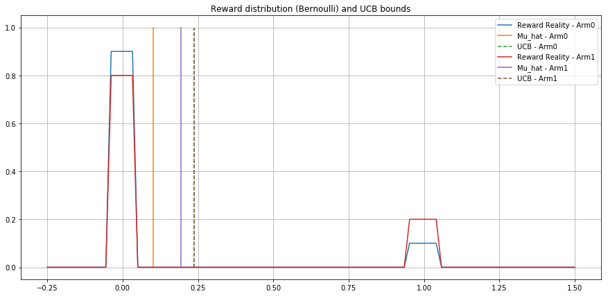
Agent UCB
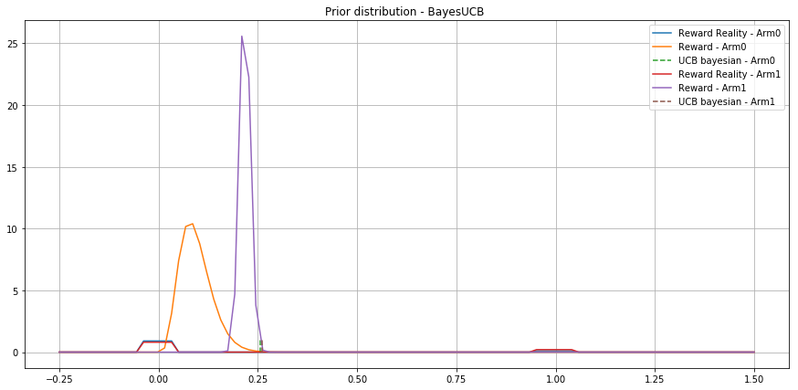
Agent UCB-Bayes
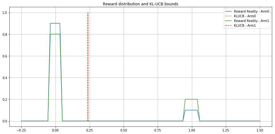
Agent KL-UCB
Expected Cumulative
Reward
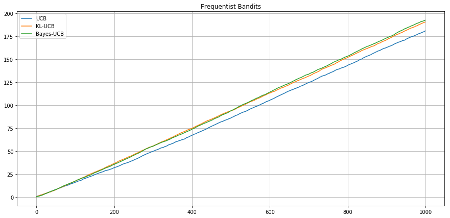
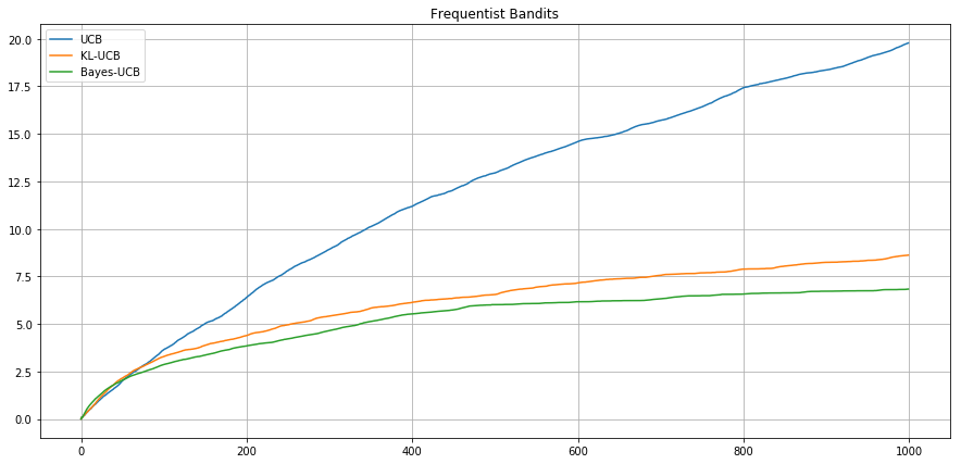
Expected Cumulative
Regret
Numerical Results
Frequentist setting - Bernoulli - .1 vs .2 -
Numerical Results
Frequentist setting - Bernoulli (0.1, 0.3, 0.55, 0.56)
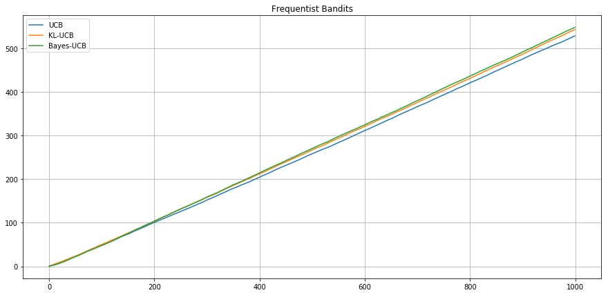
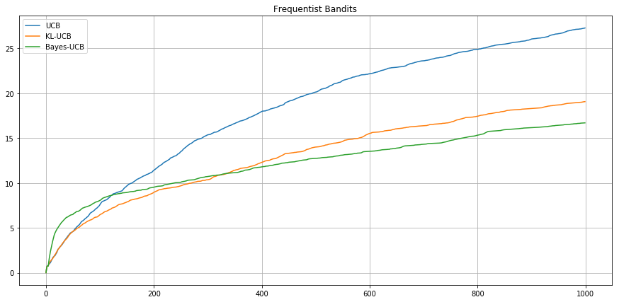
Expected Cumulative
Regret
Expected Cumulative
Reward
Agent UCB
Agent UCB Bayes
Numerical Results
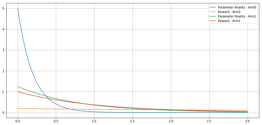
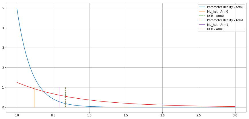
Bayesian setting - Exponential - 0.2 vs 0.8 -
Expected Cumulative
Reward
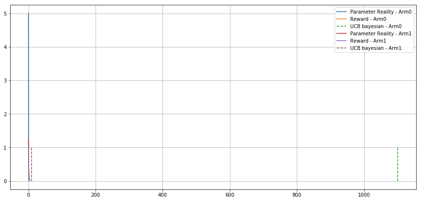
Odd behavior
95% quantile is higher for the distribution with lower expectation
Numerical Results
Bayesian setting - Exponential - 0.2 vs 0.8 -
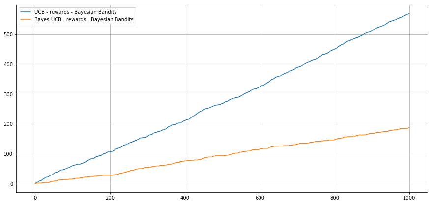
Expected Cumulative
Reward
Numerical Results
Bayesian setting - Bernoulli - Beta(2;1) vs Beta(3;1)
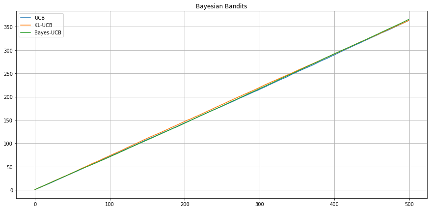
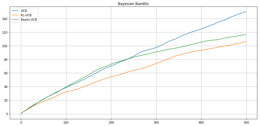
Expected Cumulative
Regret
Expected Cumulative
Reward
Numerical Results
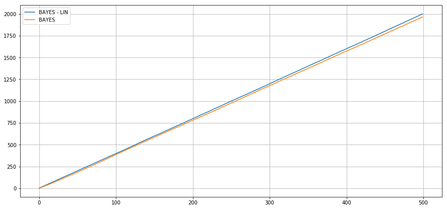
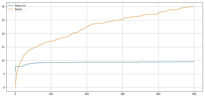
Bayesian setting - Linear rewards
Expected Cumulative
Regret
Conclusion
- New setting (generalisation of the setting seen in class).
- An efficient algorithm in frequentist bandits.
- Implementation of a scalable framework (in Python) for stochastic bandits problem (Bayesian & Frequentist)
- Broader modelisation spectrum allows easier tuning to real use cases