Custom PyMC3 nonparametric Bayesian models built on top of the scikit-learn API
Daniel Emaasit
Data Scientist
Haystax Technology
Bayesian Data Science DC Meetup
October 11, 2018


Materials
Download slides & code:


Application (1/3)


- Optimizing complex models in autonomous vehicles.


Application (2/3)


- Automating machine learning


Application (3/3)


- Supplying internet to remote areas


Intro to Bayesian Nonparametrics


Bayesian Nonparametrics (1/2)
- Task: Function approximation.
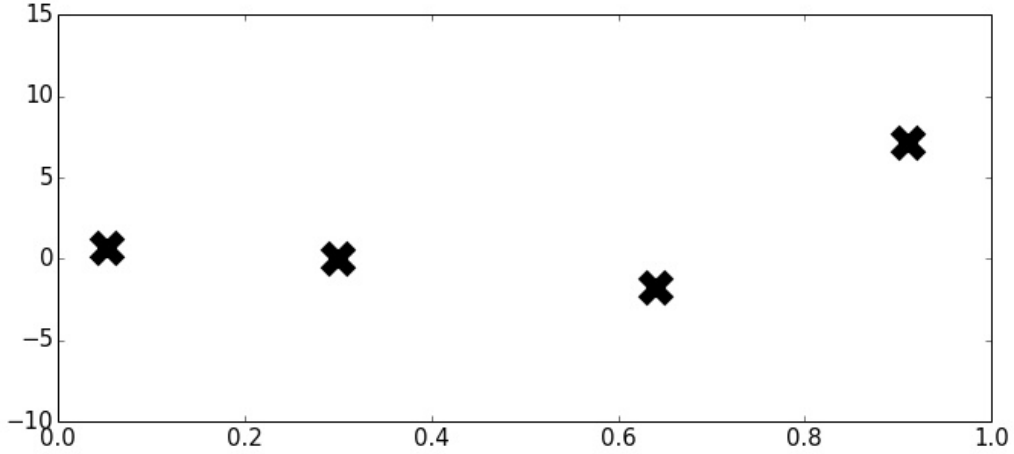
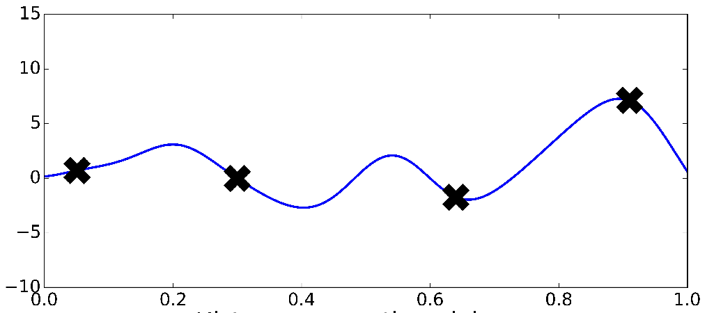
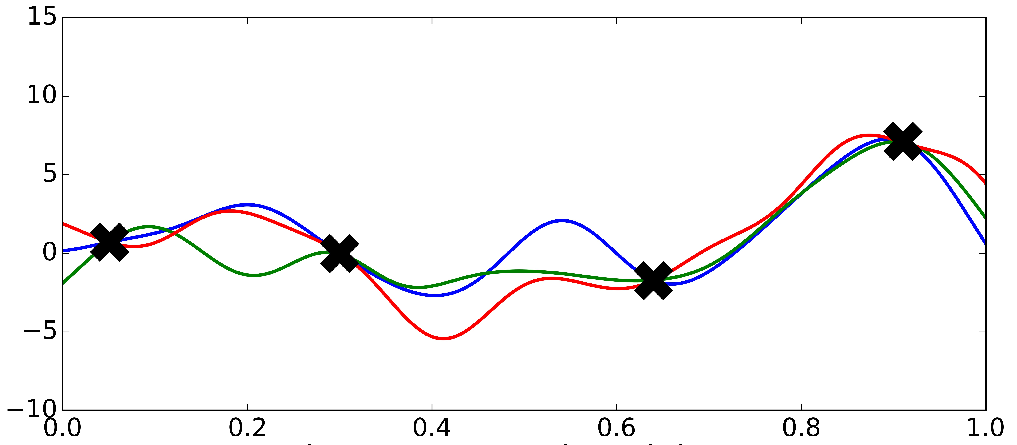
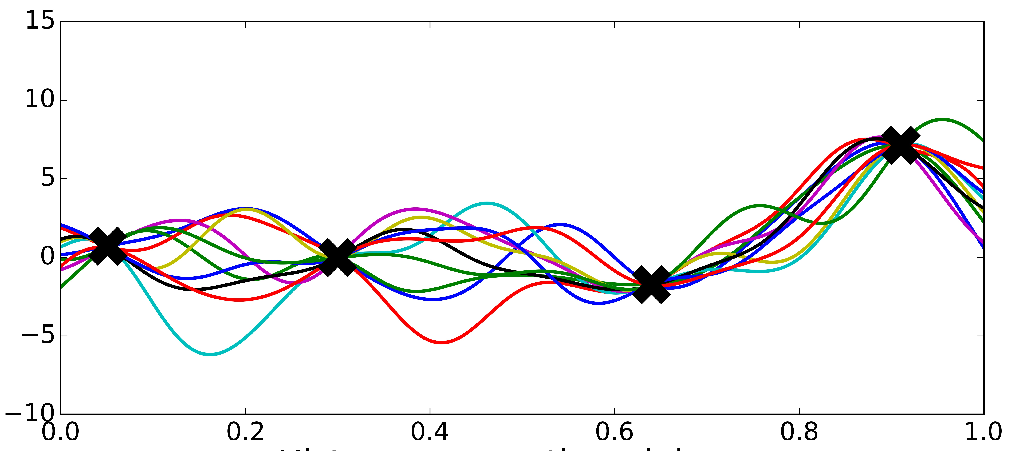
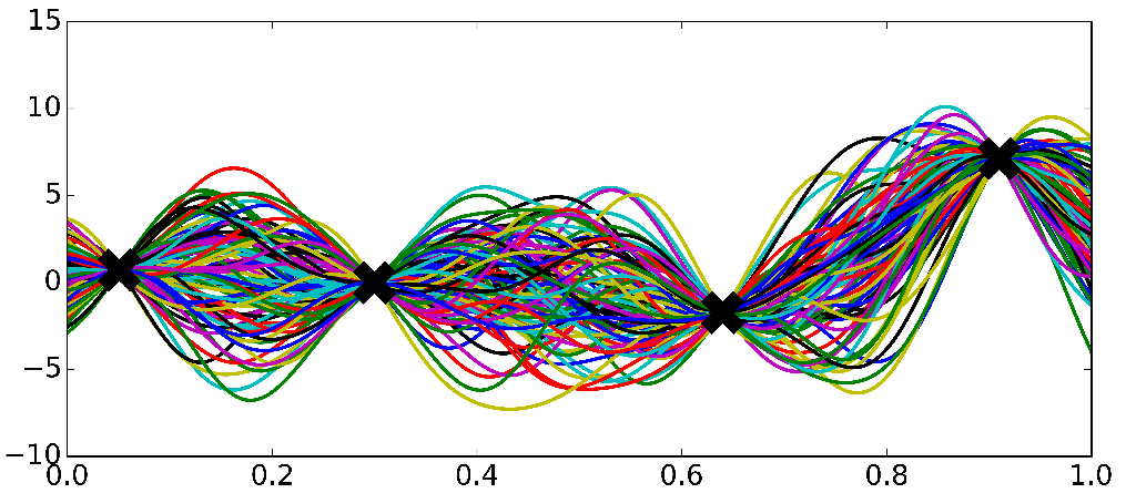
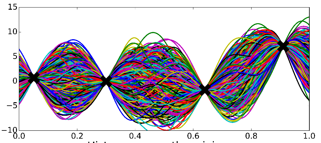
3. pre-specifying \(f(\textbf{X})\) may produce either overly complex or simple models
- Most approaches to modeling focus on parametric models that impose restrictive assumptions, e.g:
2. it's difficult to know a priori the most appropriate number of parameters
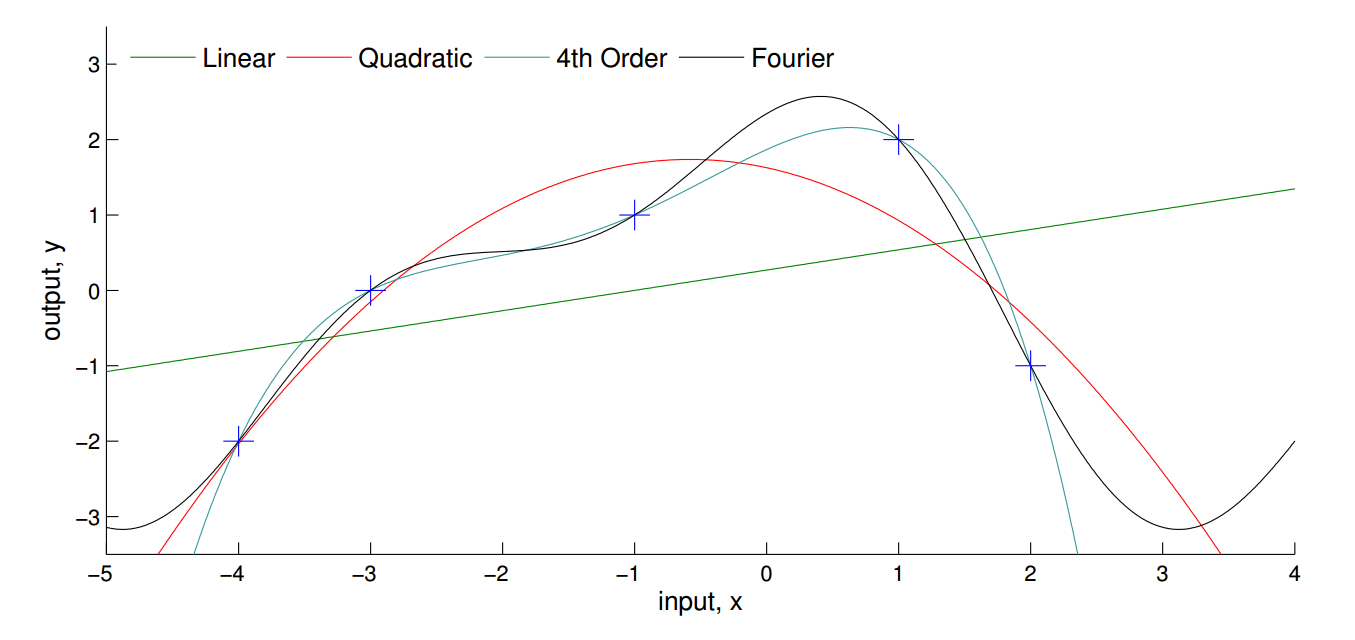
- Limitations of this approach:
- prespecifying the functional form,
2. prespecifying the number of parameters, e.g \( \text{coefficients }\beta, \text{variance }\sigma^2 \)
1. it's difficult to know a priori the most appropriate function
Or
Bayesian Nonparametrics (2/2)


Gaussian Process
- Methods that require weaker or less restrictive assumptions are preferred.
- leads to estimating flexible* models e.g Gaussian Processes
*Ghahramani, 2016
20
15
10
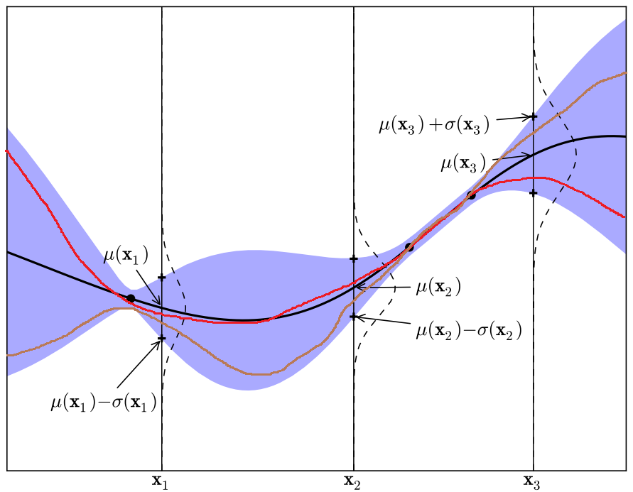
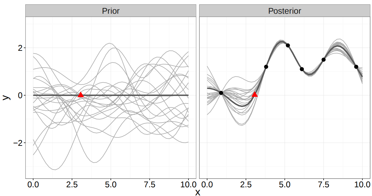
Define a prior over the function
- A distribution over functions in an infinite space is:
- a Gaussian process (GP) (Rasmussen & Williams , 2006)
where
- \(\mathbf{m}_f\) = mean function
- \(\textbf{K}_{f}\) = covariance function (kernel)

See Appendix for mathematical details
Probabilistic Programming
Probabilistic Programming (1/2)


- Probabilisic Programming (PP) Languages:
- Software packages that take a model and then automatically generate inference routines (even source code!) e.g Pyro, Stan, Infer.Net, PyMC3, TensorFlow Probability, etc.


Probabilistic Programming (2/2)


- Steps in Probabilisic ML:
- Build the model (Joint probability distribution of all the relevant variables)
- Incorporate the observed data
- Perform inference (to learn distributions of the latent variables)

Gaussian Process in PyMC3


import pymc3 as pm

# Instantiate a model
with pm.Model() as latent_gp_model:

    # specify the priors
    length_scale = pm.Gamma("length_scale", alpha = 2, beta = 1)
    signal_variance = pm.HalfCauchy("signal_variance", beta = 5)
    noise_variance = pm.HalfCauchy("noise_variance", beta = 5)
    degrees_of_freedom = pm.Gamma("degrees_of_freedom", alpha = 2, beta = 0.1)

    # specify the kernel function
    cov = signal_variance**2 * pm.gp.cov.ExpQuad(1, length_scale)

    # specify the mean function
    mean_function = pm.gp.mean.Zero()

    # specify the gp
    gp = pm.gp.Latent(cov_func = cov)

    # specify the prior over the latent function
    f = gp.prior("f", X = X)

    # specify the likelihood
    obs = pm.StudentT("obs", mu = f, lam = 1/signal_variance, nu = degrees_of_freedom, observed = y)
# Perform Inference
with latent_gp_model:
    posterior = pm.sample(draws = 100, njobs = 2)
# extend the model by adding the GP conditional distribution so as to predict at test data
with latent_gp_model:
    f_pred = gp.conditional("f_pred", X_new)

# sample from the GP conditional posterior
with latent_gp_model:
    posterior_pred = pm.sample_ppc(posterior, vars = [f_pred], samples = 200)
Build a model
Train a model
Prediction
Scikit-learn


from sklearn.gaussian_process import GaussianProcessRegressor()

model = GaussianProcessRegressor()

model.fit(X_train, y_train)

model.predict(X_test, y_test)

model.score(X_test, y_test)

model.save('path/to/saved/model')
Few lines of code
- Build + Train + predict + score + save + load
Pymc-learn


Pymc-learn


from pmlearn.gaussian_process import GaussianProcessRegressor()

# Instantiate a PyMC3 Gaussian process model
model = GaussianProcessRegressor()

# Fit using MCMC or Variational Inference
model.fit(X_train, y_train)

model.predict(X_test, y_test)

model.score(X_test, y_test)

model.save('path/to/saved/model')
Few lines of code
PyMC3 vs Pymc-learn


import pymc3 as pm

# Instantiate a model
with pm.Model() as latent_gp_model:

    # specify the priors
    length_scale = pm.Gamma("length_scale", alpha = 2, beta = 1)
    signal_variance = pm.HalfCauchy("signal_variance", beta = 5)
    noise_variance = pm.HalfCauchy("noise_variance", beta = 5)
    degrees_of_freedom = pm.Gamma("degrees_of_freedom", alpha = 2, beta = 0.1)

    # specify the kernel function
    cov = signal_variance**2 * pm.gp.cov.ExpQuad(1, length_scale)

    # specify the mean function
    mean_function = pm.gp.mean.Zero()

    # specify the gp
    gp = pm.gp.Latent(cov_func = cov)

    # specify the prior over the latent function
    f = gp.prior("f", X = X)

    # specify the likelihood
    obs = pm.StudentT("obs", mu = f, lam = 1/signal_variance, nu = degrees_of_freedom, observed = y)


# Perform Inference
with latent_gp_model:
    posterior = pm.sample(draws = 100, njobs = 2)

# extend the model by adding the GP conditional distribution so as to predict at test data
with latent_gp_model:
    f_pred = gp.conditional("f_pred", X_new)

# sample from the GP conditional posterior
with latent_gp_model:
    posterior_pred = pm.sample_ppc(posterior, vars = [f_pred], samples = 200)
from pmlearn.gaussian_process import GaussianProcessRegressor()
# Instantiate a PyMC3 Gaussian process model
model = GaussianProcessRegressor()
# Fit using MCMC or Variational Inference
model.fit(X_train, y_train)
model.predict(X_test, y_test)Few lines of code
Many lines of code
PyMC3
Pymc-learn
Demo
Resources to get started


- Winn, J., Bishop, C. M., Diethe, T. (2015). Model-Based Machine Learning. Microsoft Research Cambridge.
- R. McElreath (2012) Statistical Rethinking: A Bayesian Course with Examples in R and Stan (& PyMC3 & brms too)
- Probabilistic Programming and Bayesian Methods for Hackers: Fantastic book with many applied code examples.
Thank You!


Appendix
Start with an inflexible* model
- Consider for each data input, \(i\), that:
\(y_i\) = output variable,
\(\mathbf{x}_i\) = covariates with dimension \(D\), e.g {income, employment, trip distance, etc}
\(f(\mathbf{x}_i)\) = function that maps \(\mathbf{x}_i\) to \(y_i\),
\(\varepsilon_i\) = noise term,
\(p(\mathbf{\theta} \mid \textbf{y},\textbf{X})\) = posterior over the parameters, given observed data
\(p(\textbf{y} \mid \mathbf{\theta},\textbf{X})\) = likelihood of output variable, given covariates & parameters
\(p(\mathbf{\theta})\) = prior over the parameters
\(p(\textbf{y} \mid \textbf{X})\) = data distribution to ensure normalization
- Bayesian modeling involves:
where
- \(\mathbf{\theta}\) = parameters e.g. coefficients
*Ghahramani, 2016; Williams & Rasmussen, 2006
Extension to a flexible* model
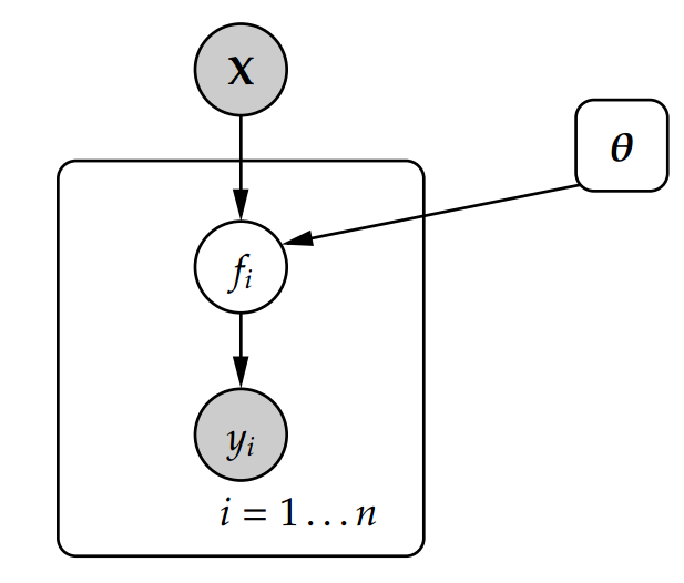
- Given that latent function \(f\), is unknown:
- It (\(f\)) is considered the parameter of interest.
\(p(\mathbf{f} \mid \textbf{y},\textbf{X})\) = posterior over the function, given observed data
\(p(\textbf{y} \mid \mathbf{f},\textbf{X})\) = likelihood of output variable, given the covariates & function
\(p(\mathbf{f})\) = prior over the function
\(p(\textbf{y} \mid \textbf{X})\) = data distribution to ensure normalization
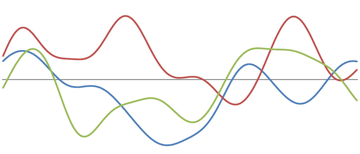
- Consider the prior over the function as:
- as any possible function in an infinite space
*Ghahramani, 2016; Williams & Rasmussen, 2006
Define a prior over the function (1/2)
- A distribution over functions in an infinite space is:
- a Gaussian process (GP) (Rasmussen & Williams , 2006)
where
- \(\mathbf{m}_f\) = mean function
- \(\textbf{K}_{f}\) = covariance function (kernel)

Define a prior over the function (2/2)
- \(\sigma^2_f\) = signal-variance parameter
- \(l_d\) = length-scale parameter (\(l_d\) is positive; controls smoothness)
- The Squared Exponential Automatic Relevance Determination (SE-ARD) kernel (Neal, 2012).
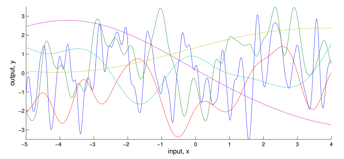
Very smooth i.e continuous
We expect our functions to vary smoothly
- Assumption:
- Recent sampling methods considered efficient in high dimensions will be used:
Efficient sampling
- Hamiltonian Monte Carlo (HMC) i.e. No-U-turn Sampler (NUTS) (Hoffman & Gelman, 2014)
- Estimation will involve finding values for two sets hyperparameters:
- \(\sigma^2_f\) & \(\sigma^2_g\) = signal-variance & noise variance
- Automatic Differentiation Variational Inference (ADVI) (Kucukelbir et al, 2016)
- \(l_d^f\) & \(l_d^g\) = length-scales in \(f\) and \(g\)
