Computational Optimization and Machine Learning

Huang Fang

June 22, 2024

Education background

Central University of Finance and Economics, 2011- 2015
- B. S. in Applied Math

University of California, Davis. 2015 - 2017
- M.S. in Statistics and Computer Science
- Worked with Prof. Cho-Jui Hsieh

University of British Columbia. 2017-2021
- Ph. D. in Computer Science
- Worked with Prof. Michael Friedlander

Industry experience

Huawei Vancouver Research Center, 2020-2021
- Developed Huawei's linear programming solver -- OptVerse;
- Research on federated learning.

Baidu, 2022 Jan -- Now.
- Research on optimization and knowledge reasoning;
- Motion prediction for auto-driving;
- Training ERNIEBot (pretraining and alignment).

Research plan

Efficient and scalable optimization algorithms
- Knowledge reasoning, language modeling, SDP, etc.

Optimization with generalization ability
- Language model alignment.

ML for algorithm discovery
- Using data-driven principle to find better algorithm, AI for math, etc.

Overview

Part I: first-order optimization
- Coordinate optimization
- Online mirror descent
- Stochastic subgradient descent

Part II: optimization for applications
- Computational optimization for knowledge reasoning
- Computational optimization for large language models

Part I: First-order methods

Optimization is everywhere: machine learning, operation research, data mining, theoretical computer science, etc.

\underset{x \in C}{\min} ~f(x)

First-order methods:

x^{(t)} = \text{span}\{ x^{(0)}, \nabla f( x^{(0)} ), \nabla f( x^{(1)} ), \ldots, \nabla f( x^{(t-1)} ) \}

Why first-order methods?

First-order method

x^{(t)}

x^{(t+1)}

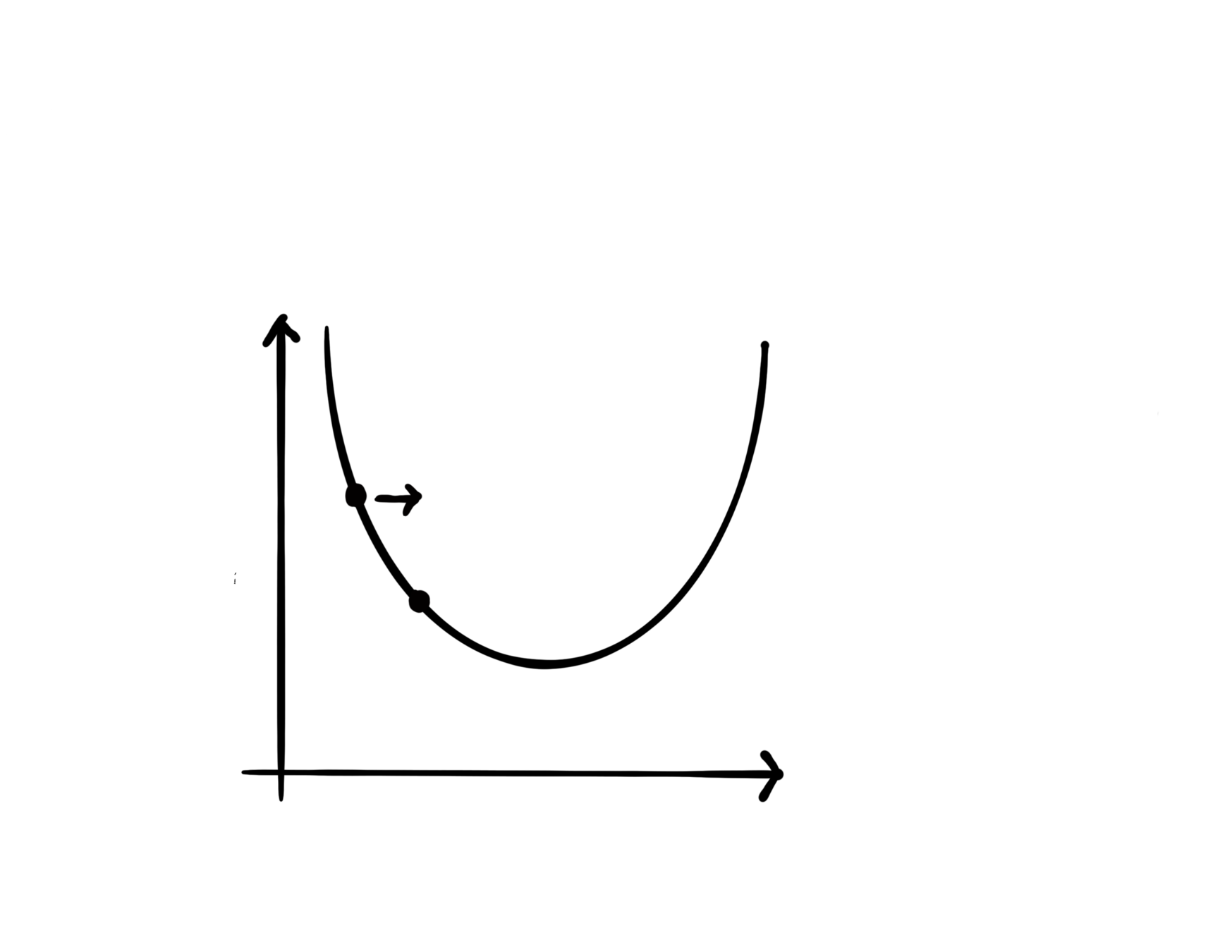
The literature

Gradient descent can be traced back to Cauchy's work in1847.

It is gaining increasing interest in the past 3 decades due to its empirical success.

Fundamental works have been done by pioneering researchers (Bertsekas, Nesterov, etc.).

There are still gaps between theory and practice.

Coordinate optimization

Mirror descent

Stochastic subgradient method

Coordinate Optimization

Coordinate Descent

For

t = 0, 1, 2, \ldots,

Select coordinate

i \in [d]

Update

x_i^{(t+1)} = x_i^{(t)} - \eta_t \nabla_i f( x^{(t)} )

Different coordinate selection rules:

Random selection:

Cyclic selection:

Random permuted cyclic (the matrix AMGM inequality conjecture is false [LL20, S20])

Greedy selection (Gauss-Southwell)

i \in \arg\max_{ j \in [d] } | \nabla_j f( x^{(t)} ) |

i \sim \mathrm{uniform}\{1,2,\ldots, d\}

i = (t-1) ~\mathrm{mod}~ d + 1

Forty-Two Open Problems in the Mathematics of Data Science

GCD for Sparse Optimization

\underset{ x \in \mathbb{R}^d }{\min}~F(x) \coloneqq f(x) + g(x)

regularizer

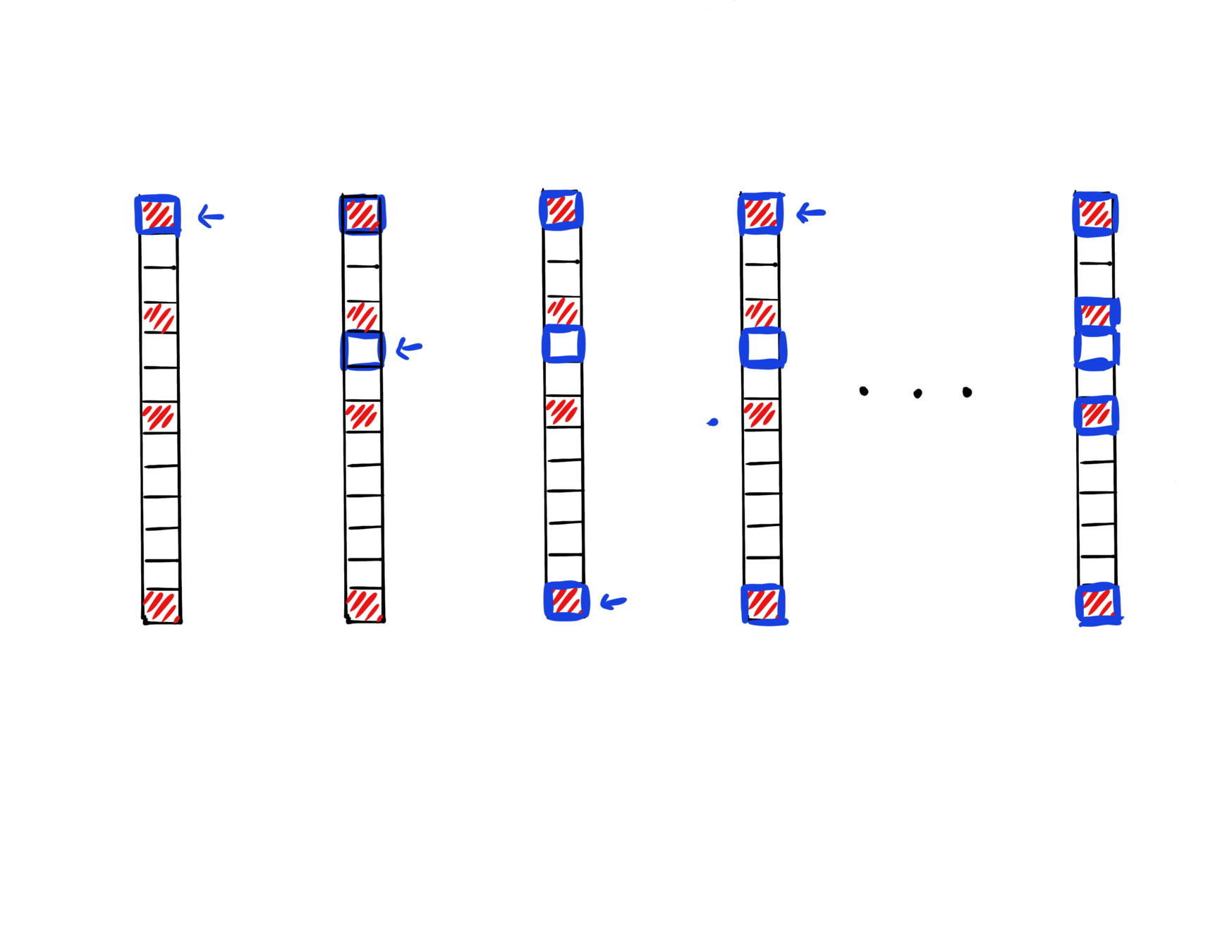
One-norm regularization or nonnegative constraint can promote a sparse solution.

When initailzed at zero, greedy CD is observed to have an implicit screening ability to select variables that are nonzero at solution.

Iter 1

Iter 2

Iter 3

Iter 4

Iter

g(x) = \lambda \| x \|_1

g(x) = \delta_{\geq 0}(x)

data fitting

GCD for Sparse Optimization

[FFSF, AISTATS'20]

We provide a theoretical characterization of GCD's screening ability:

GCD converges fast in first few iterations.

The iterate is "close" the to solution when the iterate is still sparse, and sparsity pattern will not further expand anymore.

x^{(0)}

x^{*}

x^{(100)}

d = 10^4, \| x^* \|_0 = 10

\| x^{(t)} \|_0 \leq 110

for

t > 100

\delta

From coordinate to atom

Learning a sparse representation of an atomic set :

\mathcal{A}

x^* = \sum_{a \in \mathcal{A}} c_a a

such that

c_a \geq 0~\forall a \in \mathcal{A}.

sparse vector:

\mathcal{A} = \{ \pm e_1, \pm e_2, \ldots, \pm e_d \}

Low-rank matrix:

\mathcal{A} = \{ uv^T \mid u \in \mathbb{R}^{n}, v \in \mathbb{R}^m, \|u\| = \|v\| = 1 \}

Our contribution: how to identify the atoms with nonzero coefficients at solution during the optimization process.

[FFF, OJMO'24]

Online Mirror Descent

Online Convex Optimization

Play a game for rounds, for

Propose a point

x^{(t)} \in \mathcal{X}.

Suffer loss

f_t( x^{(t)} ).

t = 1,2,\ldots, T

The goal of online learning algorithm: obtain sublinear regret

\displaystyle \mathrm{Regret} (T, z) \coloneqq \sum_{t=1}^T f_t( x^{(t)} ) - \sum_{t=1}^T f_t(z).

\mathrm{Regret} (T, z) = o(T) \to \mathrm{Regret} (T, z)/T \to 0.

player's loss

competitor's loss

Mirror Descent (MD) and Dual Averaging (DA)

MD and DA are parameterized by mirror map, they have advantages over the vanilla projected subgradient method.

f_t(x) = c_t^T x \quad \text{and} \quad \mathcal{X} = \left\{ \sum_{i=1}^d x_i = 1, x_i \geq 0 \right\}, ~\|c_t\|_{\infty} \leq 1.

When is known in advance or , both MD and DA guarantee regret

\mathcal{O}( \sqrt{T} ).

When is unknown in advance and , then MD has rate while DA still guarantees regret.

\sup_{x, y \in \mathcal{X}} D_\Phi(x, y) = +\infty

\Omega ( T )

\mathcal{O}( \sqrt{T} )

\sup_{x, y \in \mathcal{X}} D_\Phi(x, y) < +\infty

Our contribution: fix the divergence issue of MD and obtain

regret.

\mathcal{O}( \sqrt{T} )

OMD Algorithm

[FHPF, ICML'20, JMLR'22]

Primal

Dual

x^{(t)}

\hat{x}^{(t)}

\nabla \Phi

\hat{y}^{(t)}

-\eta_t \nabla f_t( x^{(t)} )

y^{(t)}

x^{(t+1)}

Bregman projection

\nabla \Phi^*

Figure accredited to Victor Portella.

Stabilized OMD

[FHPF, ICML'20, JMLR'22]

Primal

Dual

x^{(t)}

\hat{x}^{(t)}

\nabla \Phi

\hat{y}^{(t)}

-\eta_t \nabla f_t( x^{(t)} )

y^{(t)}

x^{(t+1)}

Bregman projection

\nabla \Phi^*

\hat{x}^{(0)}

\hat{w}^{(t)}

}

\gamma_t

With stabilization, OMD can obtain regret.

\mathcal{O}( \sqrt{T} )

(Stochastic) Subgradient Method

Smooth v.s. Nonsmooth Minimization

Consider minimizing a convex function

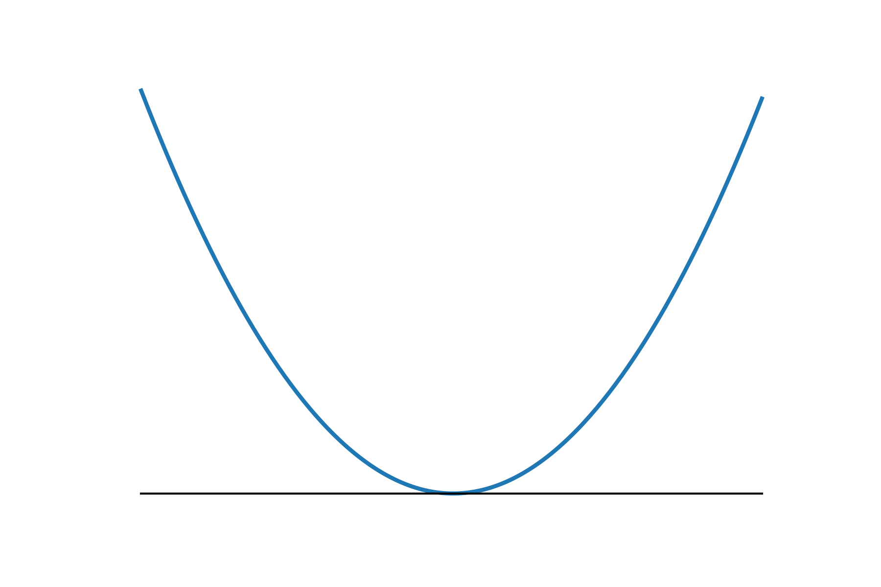
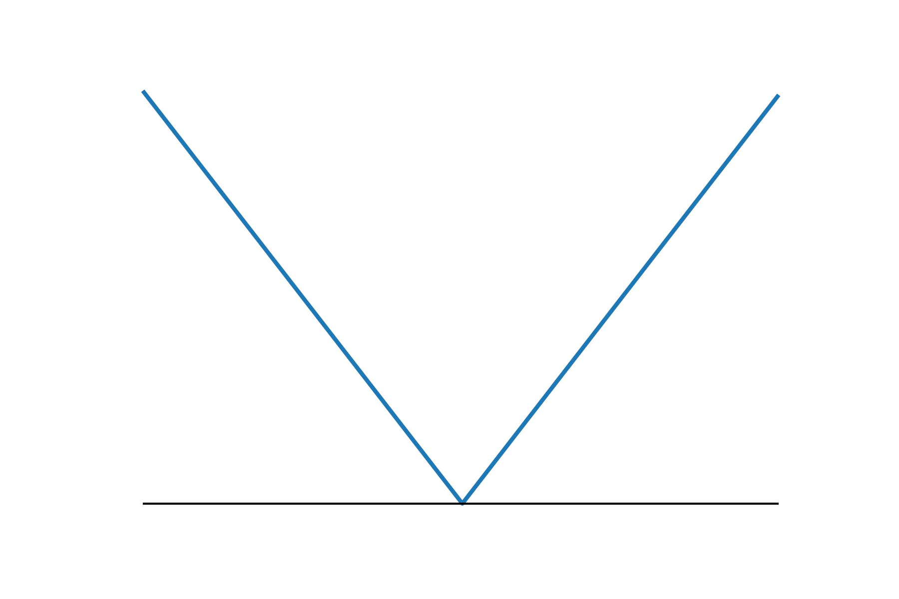
The iteration complexity of gradient descent (GD) and subgradient descent (subGD) for smooth and nonsmooth objectives:

\underset{ x \in \mathbb{R}^d }{\min}~ f(x).

when is smooth:

\mathcal{O}(1/\epsilon).

when is nonsmooth:

\mathcal{O}(1/\epsilon^2).

smooth

nonsmooth

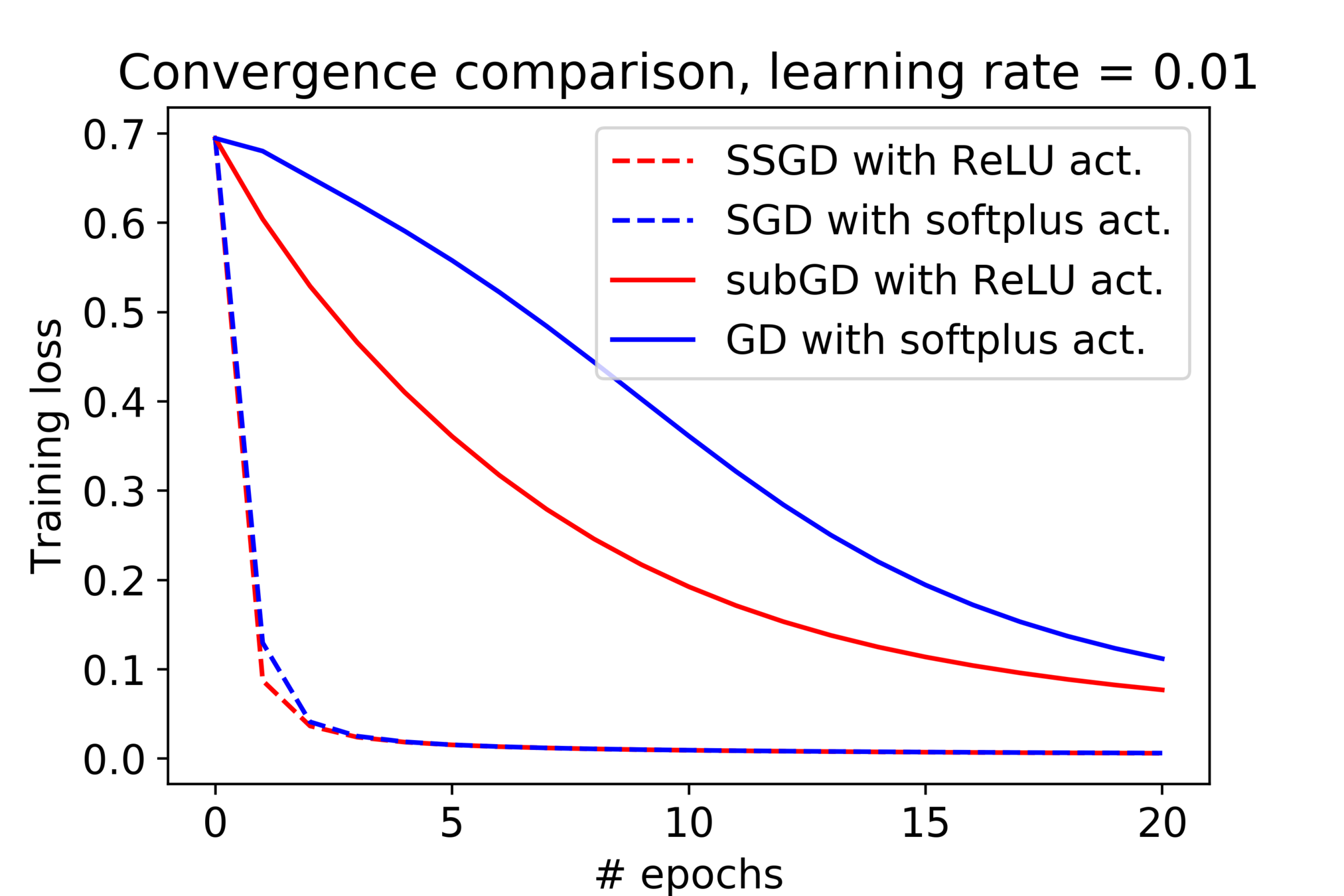
The empirical observation

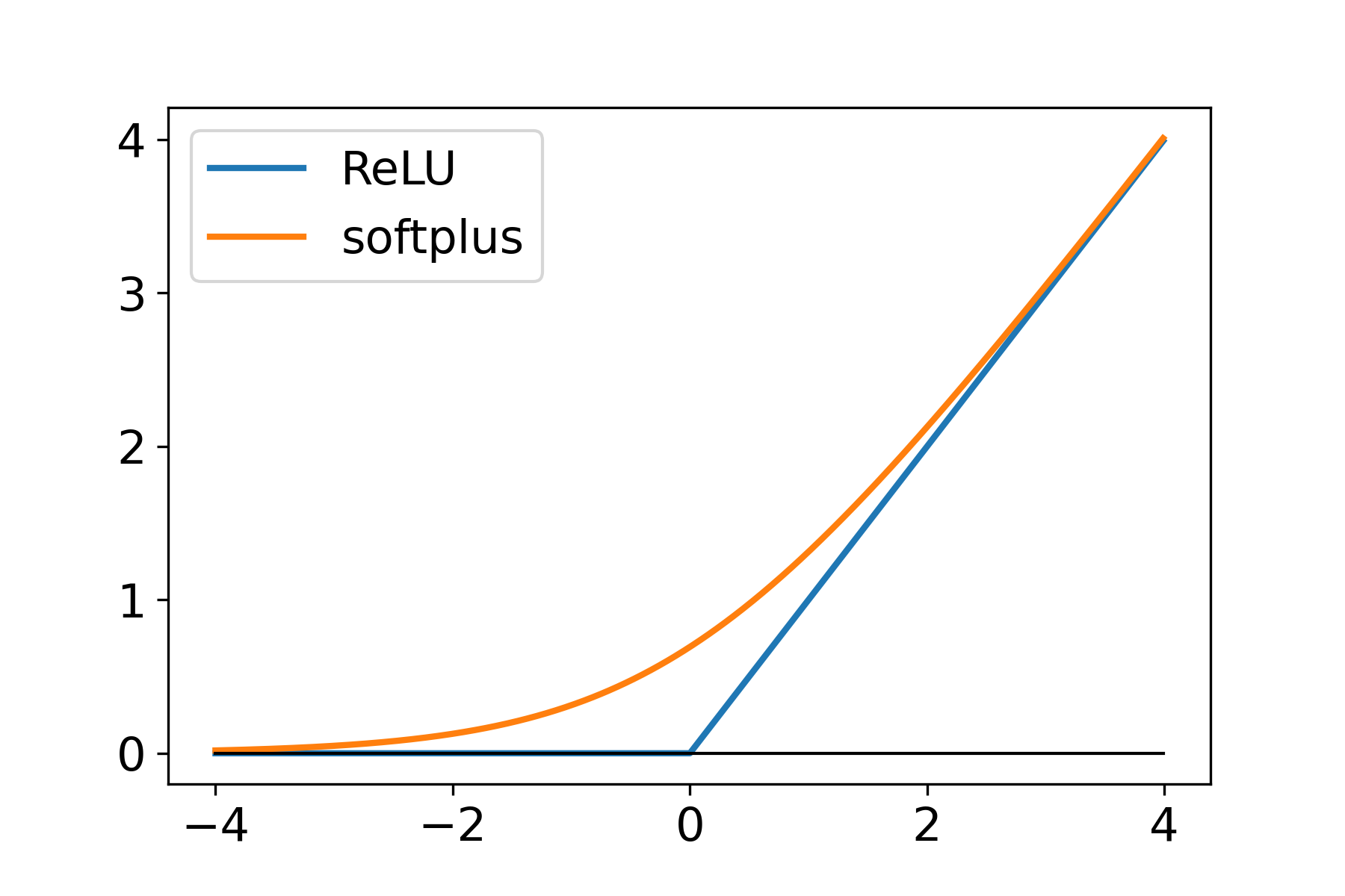
Some discrepancies between theory and practice:

Nonsmoothness from the model does not slow down our training in practice.

The learning rate schedule can yield optimal iteration complexity but seldom used in practice.

\eta_t \propto 1/\sqrt{t}

Filling the gap

Two important structures:

The objective satisfy certain structure:

\underset{x \in \mathbb{R}^d}{\min}~ f(x) = \frac{1}{n} \sum_{i=1}^n f_i(x) \coloneqq \frac{1}{n} \sum_{i=1}^n \ell(h_i(x)),

where is a nonnegative, , convex, 1-smooth loss function, 's are Lipschitz continuous.

\ell : \mathbb{R} \to \mathbb{R}_{\geq 0}

The interpolation condition: there exist such that

x^*

f(x^*) = 0 .

h_i

[FFF, ICLR'21]

\inf \ell = 0

square loss, L2-hinge loss, logistic loss, etc.

absolute loss, L1-hinge loss.

Filling the gap

With constant learning rate, we prove

Convex objective:

Strongly convex objective:

\mathcal{O}(1/\epsilon^2) \to \mathcal{O}(1/\epsilon).

\mathcal{O}(1/\epsilon) \to \mathcal{O}(\log(1/\epsilon)).

The above rates match the rate of SGD for smooth objectives.

[FFF, ICLR'21]

Lower bounds

Can we accelerated SSGD using momentum under interpolation? e.g.,

Two follow up questions:

\mathcal{O}(\epsilon^{-{1}/{2}}).

The structure stays in the center of our analysis, could this structure itself give us improved rate without the interpolation condition?

[FFF, ICLR'21]

f_i = \ell \circ h_i

The answer to above questions is "no".

With interpolation condition:

Without interpolation condition:

\mathcal{\Omega}(1/\epsilon).

\mathcal{\Omega}(1/\epsilon^2).

We derive lower bounds for iteration complexity:

Part II: Optimization for applications

Knowledge Graph Reasoning

Knowledge graph

Knowledge graph: a set of triplets , such as (Tom, workAt, Baidu), (Beijing, cityOf, China), etc.

\{ (h_i, r_i, t_i) \}_{i=1}^n

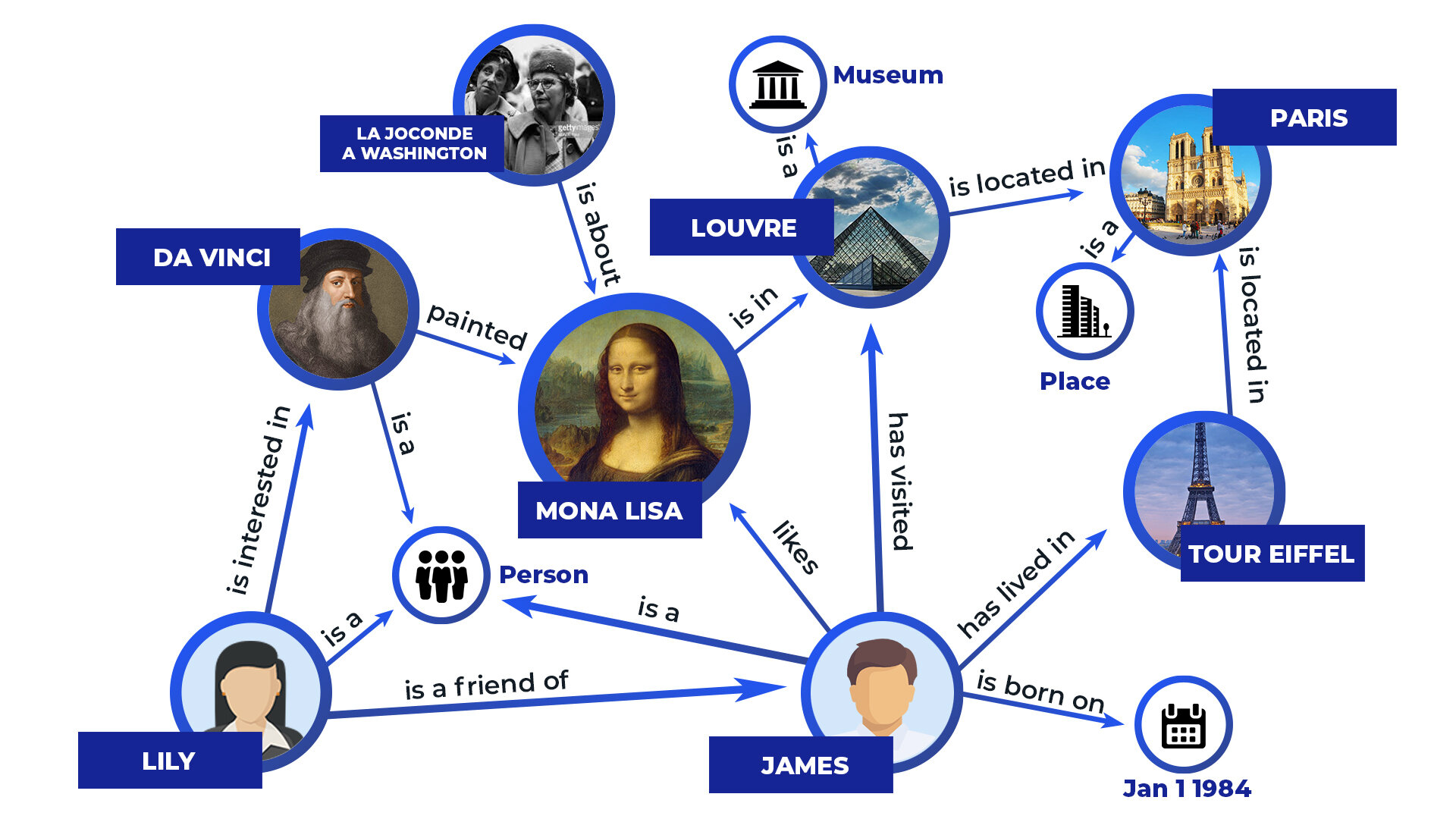
Reasoning on knowledge graph:

(h,r,?), (h, ?, t).

Markov Logic Network (MLN)

First-order logic rules:

\text{father}(X, Y) \land \text{brother}(Y, Z) \Longrightarrow \text{father}(X, Z);

\text{friend}(X, Y) \land \text{smoke}(X) \Longrightarrow \text{smoke}(Y).

1.0

0.4

Given a set of facts, MLN defines the probability of the "world" as

\displaystyle \text{Pr}(X) \propto \exp\left( \sum_{i=1}^m w_i f_i( X ) \right)

where is the number of time that the i-th rule is satisfied.

f_i(X)

The previous state of MLN

MLN suffers from an efficiency issue, both the learning and MAP inference of MLN are NP-hard.

Existing MLN solvers such as Alchemy, Tuffy, DeepDive and PSL all cannot scale to medium-size KBs.

Key insights

The MAP inference of MLN is essentially solving a huge SAT problem (potentially solved by the WalkSAT algorithm).

Expolit the sparsity of knowledge graph and develop a smart implementation of the WalkSAT algorithm.

Our implementation is based on Julia, available at https://github.com/baidu-research/MLN4KB.

[FLCS, WWW'23]

Experiments

Efficiency on the Kinship dataset.

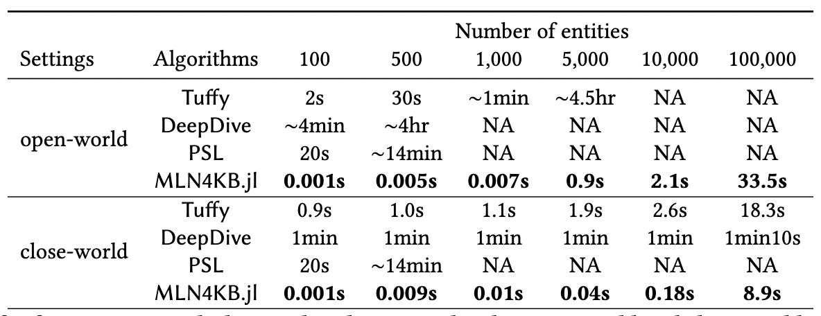
~10,000 speed up!

[FLCS, WWW'23]

Experiments

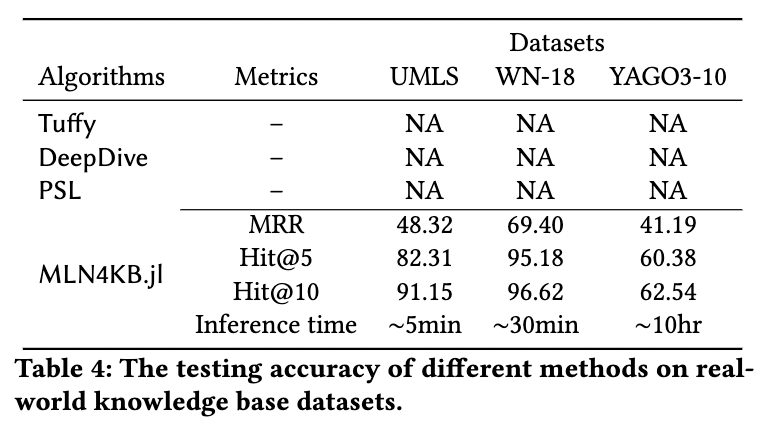
Performance on real-world KG datasets, rules extracted by the AMIE (GTHS13) software.

Memory usage:

[FLCS, WWW'23]

Follow up work

[CCFHS, NeurIPS'23]

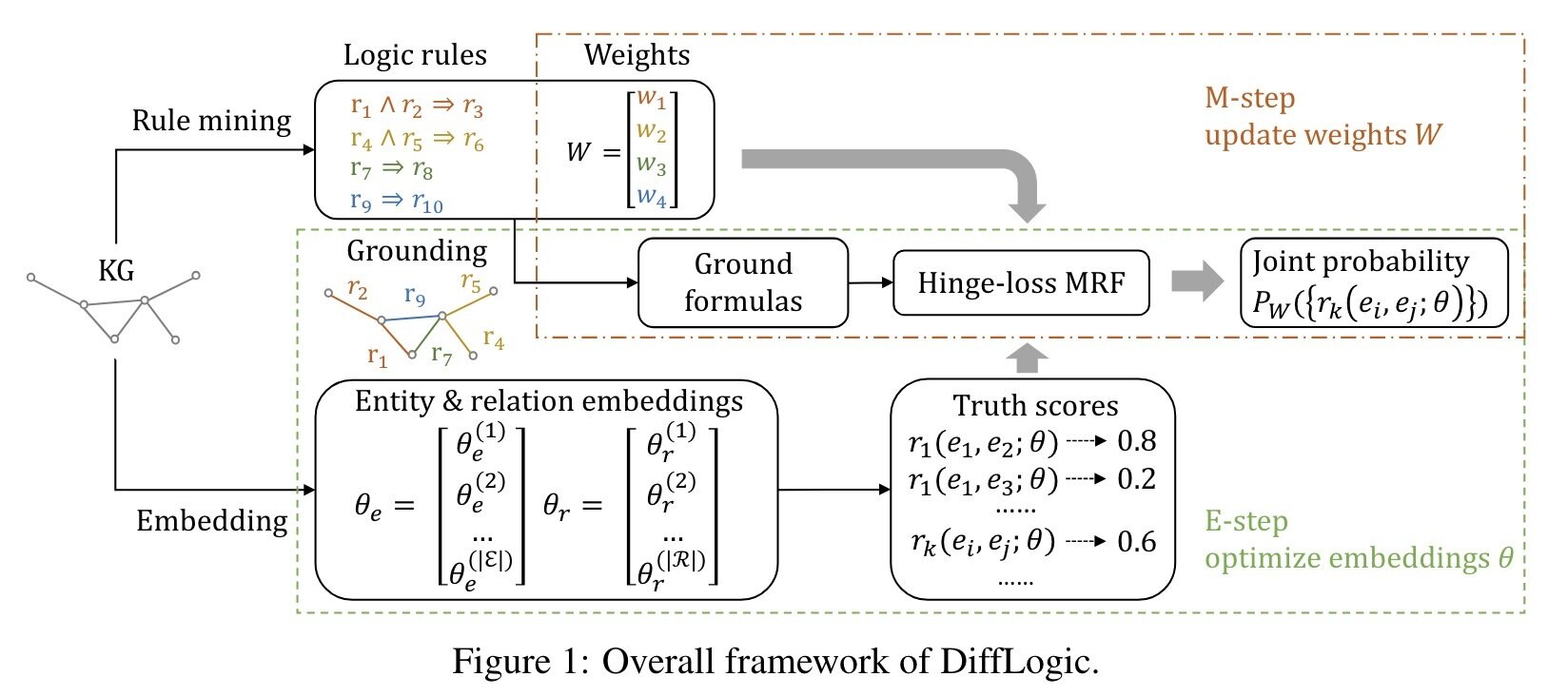
DiffLogic: combining (soft) MLN with knowledge graph embedding.

Computational Optimization and Large Language Model

Optimization matters for pretraining

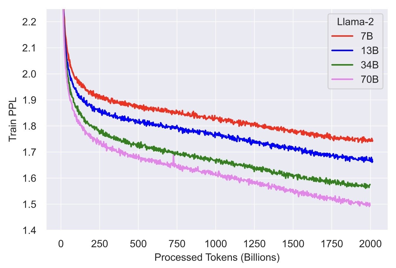
LLM pretraining is essentially an optimization problem! Lower loss means better performance.

Figure comes from "Llama 2: Open Foundation and Fine-Tuned Chat Models"

Training stability of the Adam optimizer

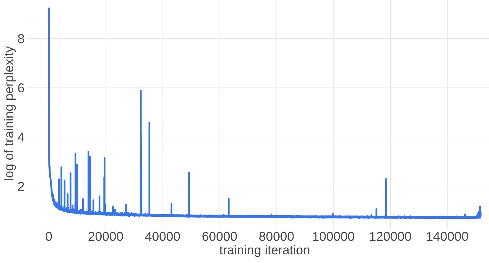
The training curve of a 546b model from META.

Figure comes from "A Theory on Adam Instability in Large-Scale Machine Learning"

Low precision training

A well-known trend: model gets larger, dataset gets larger...

A less well-known trend: float32 -> float16 -> bfloat16 -> int8 -> int4...

training

inference

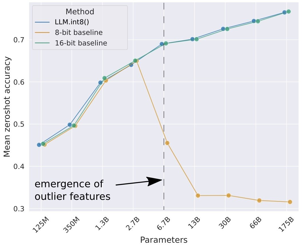
Figure comes from "LLM.int8(): 8-bit Matrix Multiplication for Transformers at Scale"

Thank you! Questions?

Matrix AMGM inequality

\displaystyle \left\| \frac{1}{n!} \sum_{ \sigma \in \mathrm{Perm}(n) } \prod_{j=1}^n A_{\sigma(j)} \right\| \leq \displaystyle \left\| \frac{1}{n^n} \sum_{ k_1,\ldots,k_n=1 }^n \prod_{j=1}^n A_{k_j} \right\|

for all PSD matrix

A_1, \ldots, A_n \in \mathbb{R}^{d \times d}.

The matrix AMGM inequality conjecture is false [LL20, S20])

Backup slides for SGD

Basics

	smooth	nonsmooth	smooth+IC	nonsmooth + IC
convex
strong cvx

\mathcal{O}(1/\epsilon)

\mathcal{O}(1/\epsilon^2)

\mathcal{O}(1/\epsilon)

\mathcal{O}(\log(1/\epsilon))

\mathcal{O}(1/\epsilon^2)

\mathcal{O}(1/\epsilon)