Dimentionality reduction and classification over MRI anatomical images using PCA
What is Dimensionality Reduction?
- Too many features while the availability of training examples is not infinite
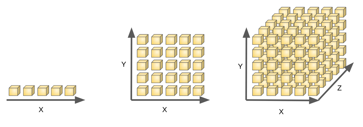
E.g. 3D Image processing 256*256*256 = 16777216 features
- As the number of feature or dimensions grows, the amount of data we need to generalise accurately grows exponentially.
- Sometimes, most of these features are correlated and hence redundant
- Feature selection & Feature extraction
Avoid curse of dimensionality:
- Reduce computational time and space required
- Ease of fitting models with high accuracy (bye to over-fitting)
- Possibility to visualize the data when reduced to 2D or 3D
Some dimensionality reduction techniques:
- ICA (independent source finding)
- SVD (efficient computation of PCA)
- PCA (correlated variables to linearly uncorrelated variables)
Why dimensionality reduction...
Data & Data Structure
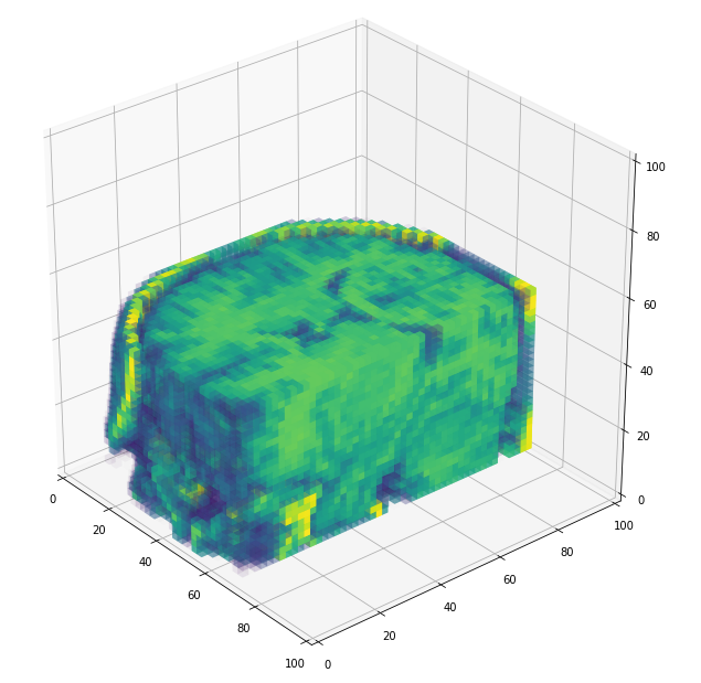
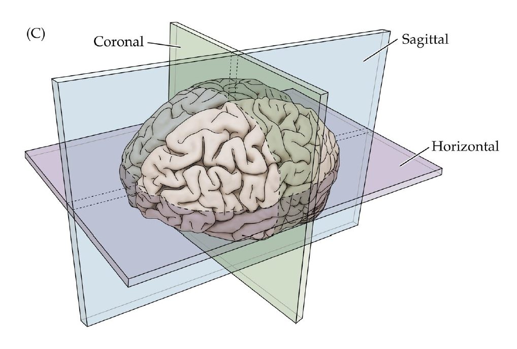
- MRI brain images (volumetric representation)
- NIfTI (.nii) files
- Size: 17.3 GB
- 1113 samples (brains)
- Preprocessed version of data
- Skull stripping.
- Normalized.
The human connectome project, 1113 subjects’ brain T1w structural images. These 3D MPRAGE (this sounds nice) images obtained from Siemens 3T platforms using a 32-channel head coil.

Cropping
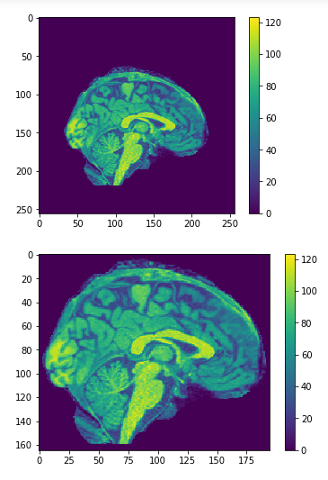
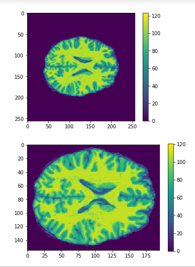
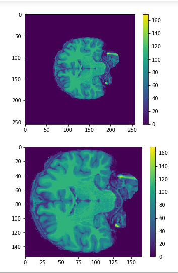
cropped = data[50:205,60:225,30:225] #155x165x195
data = img.get_data() #256x256x256
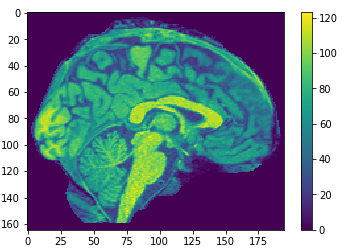
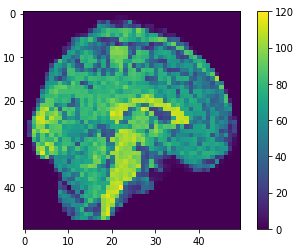
Resize
(155, 165, 195) array  #4987125 voxels
(50, 50, 50) array #125000 voxels
resampled = zoom(cropped, (50/cropped.shape[0], 50/cropped.shape[1] , 50/cropped.shape[2])
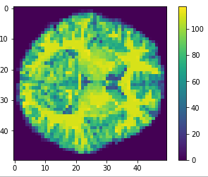
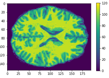
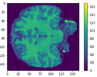
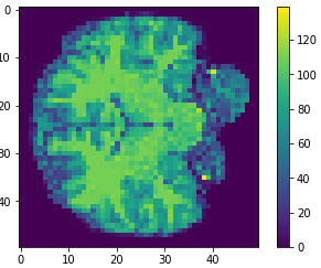
Flatten
(50, 50, 50) array #125000 voxels
vector = array.flatten()
(125000)array #125000 voxels
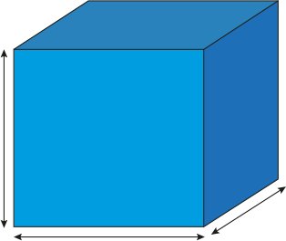


256x256x256
155x165x195
50x50x50
Original
Cropped
Resized
50x50x50
1113x125000
Save
1113 x 125000


1113
1
Flatten

file.npy
jupyter notebook
Loading, cropping , resizing and saving
50x50x50
1113x125000
ML methods


1113
1
Flatten
SVM
KNN
PCA
SVM

Principal Component Analysis
(PCA)
What is PCA
- Finding correlation between variables.
- Separating samples on a dataset.
- Eigenvalues and eigenvectors (axes of subspace)
Principal Component Analysis (PCA) is a dimension-reduction tool that can be used to reduce a large set of variables to a small set that still contains most of the information in the large set.
Visually

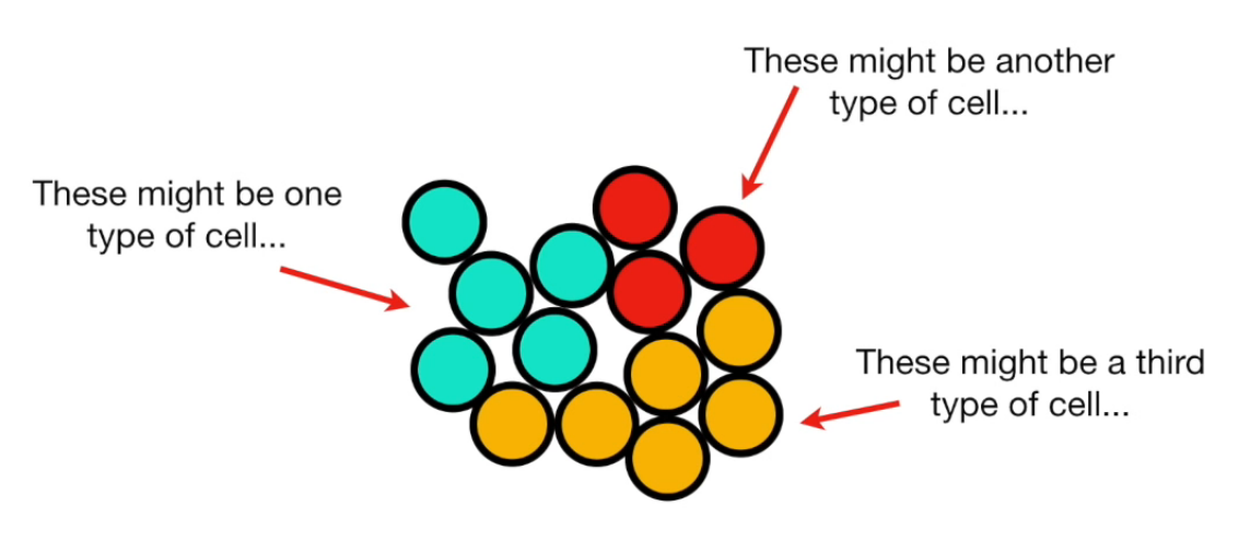
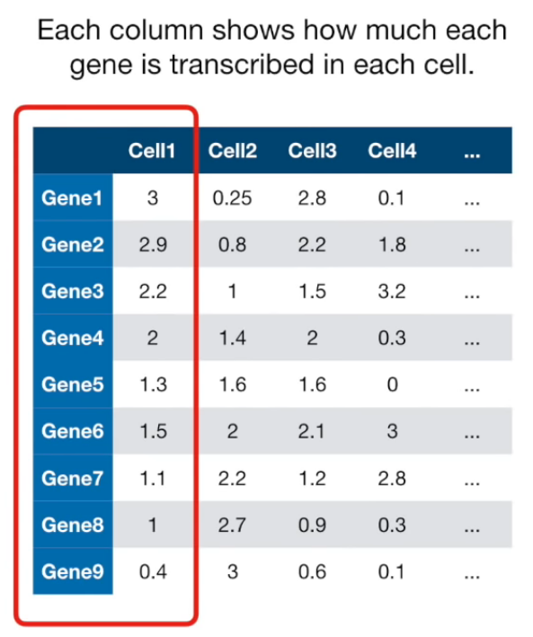
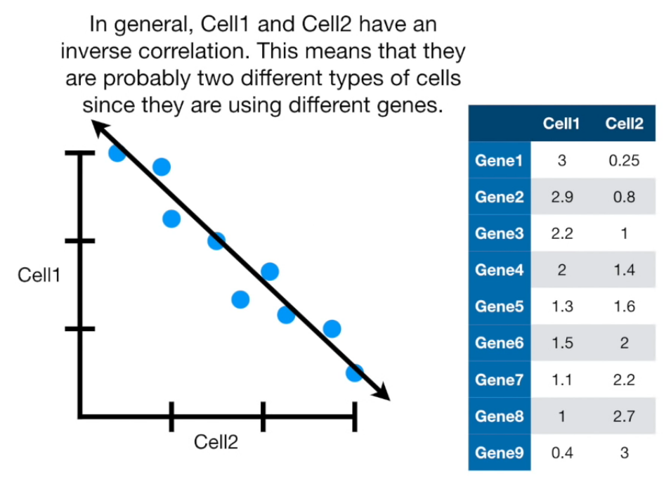
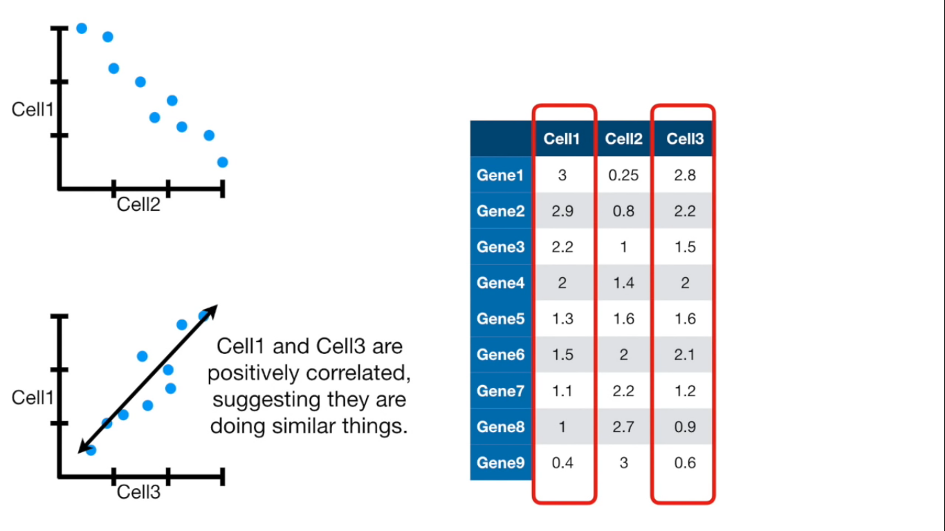
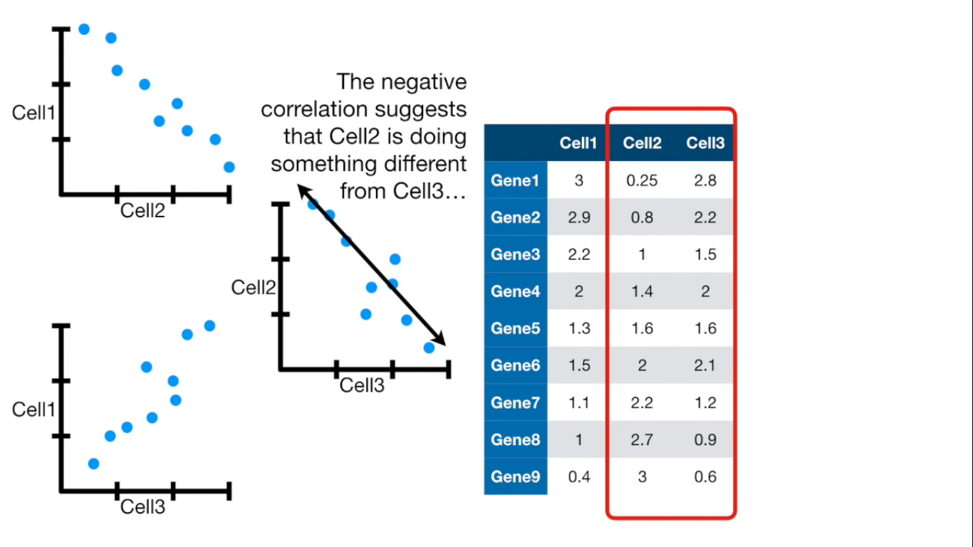
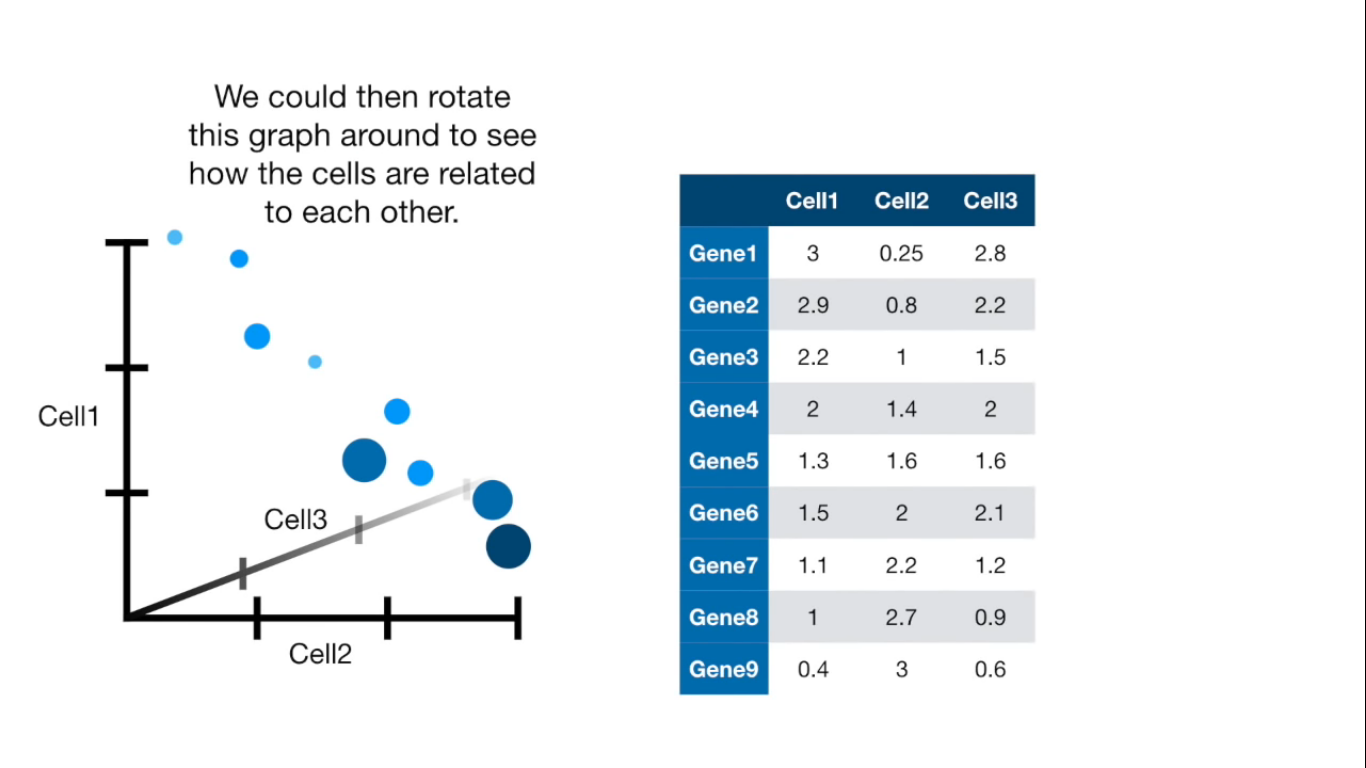
If more than 4 columns...
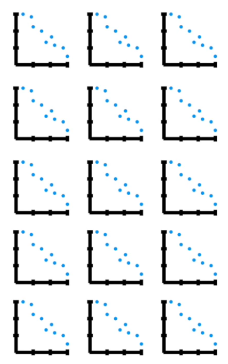
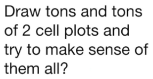
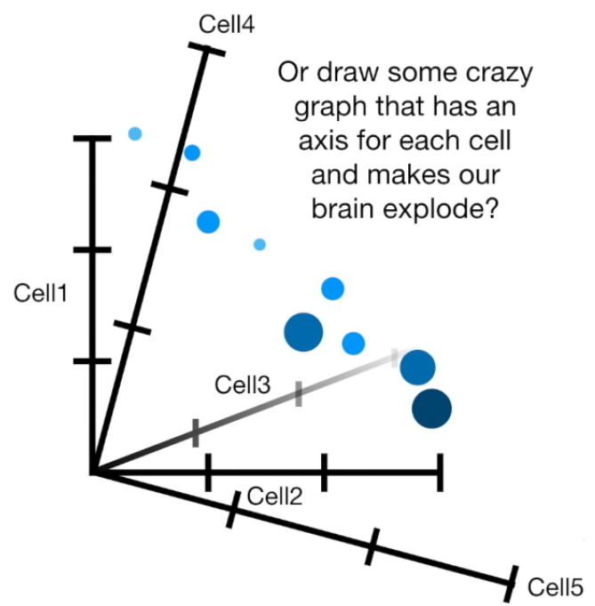
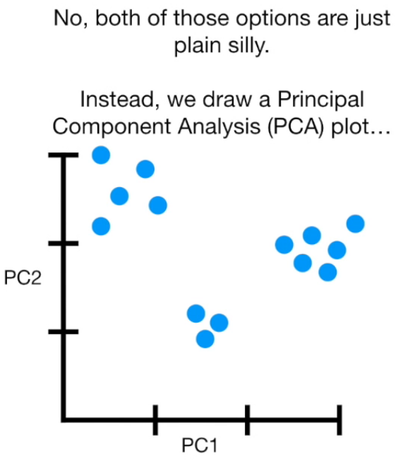
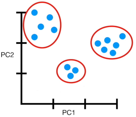
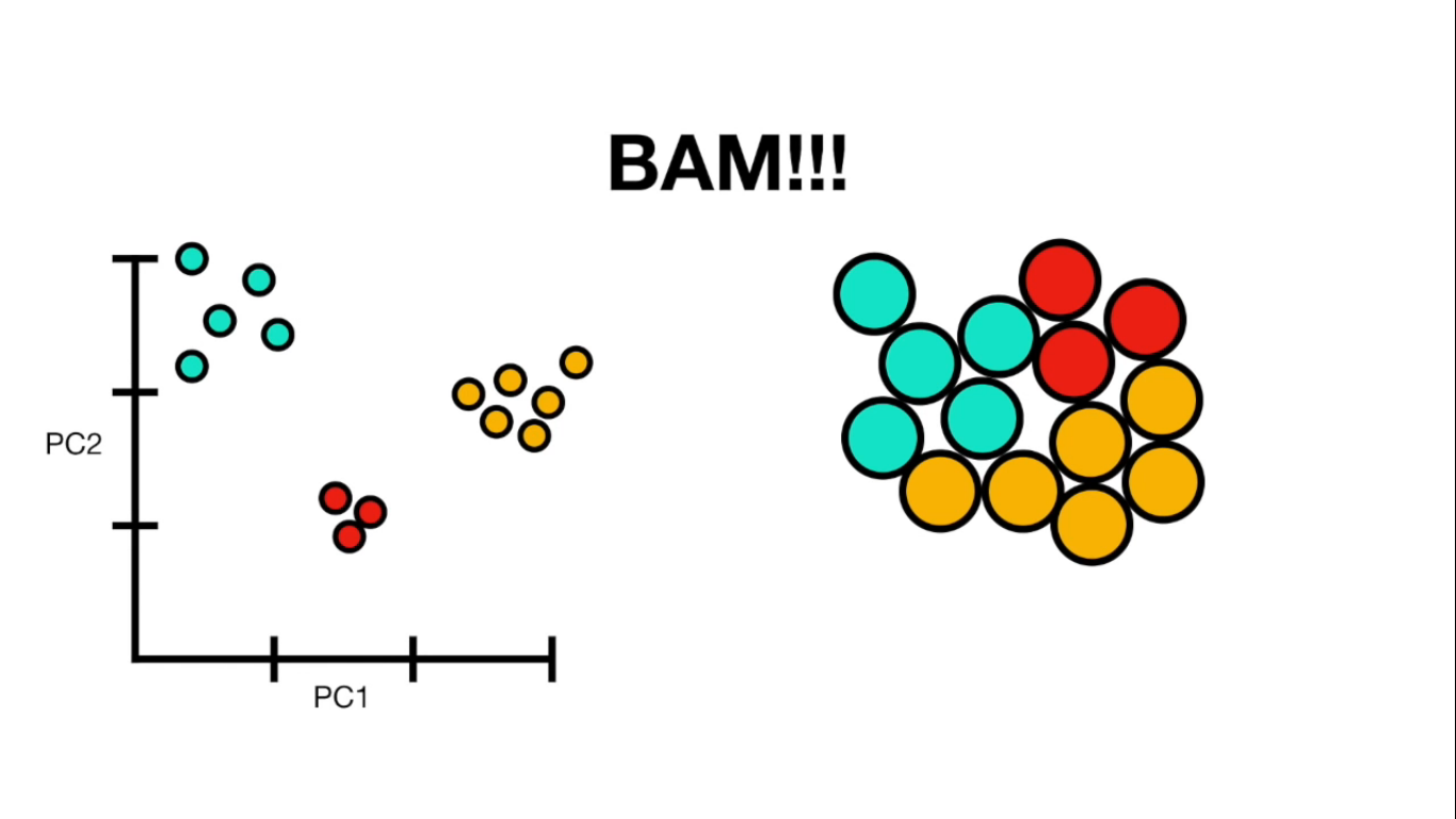
- PCA(1113x125000)
Reduce the amount of features from the original data to a serie of principal components that hold the information of the variance (axis of subspace)
EigenBrains
- (PCA(125000x1113))
Try to find a set of "standardized brain ingredients".
Feature extraction
Feature extraction
- Loading data
- Applying PCA choosing amount of components
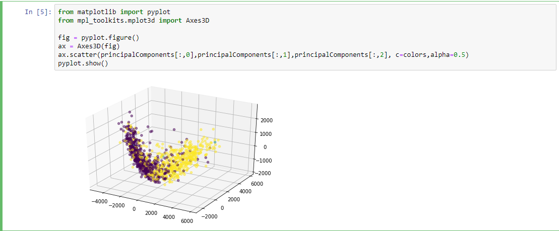
- Plotting
- Reconstructing data from components
import numpy as np
to_save_load=np.load("to_save.npy")
to_save_load.shape
(1113, 125000)
Loading data
from sklearn.decomposition import PCA
pca = PCA(n_components=10)#% of variance or number
principalComponents = pca.fit_transform(to_save_load)
(1113, 10)
Applying PCA

l = pca.explained_variance_ratio_
sum(l)#0.412558136188802
Plotting
import pandas as pd
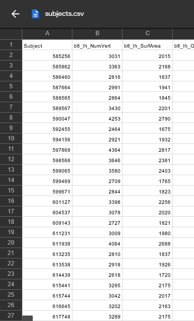
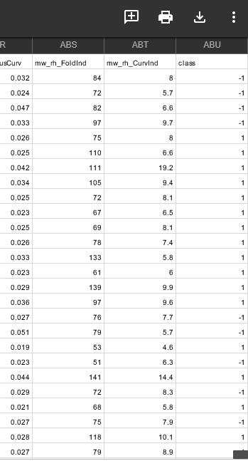
subjects = pd.read_csv('subjects.csv')
columns = subjects[['Subject','class']]
labels= columns.set_index('Subject').T.to_dict('list')
import os
dirs = os.listdir( "brain_nii" )
-
Getting Colors
{585256: [-1], 585862: [-1], 586460: [-1], 587664: [-1], 588565: [1],...}
colors = []
for name in dirs:
id,ext = name.split('.')
try:
colors.append(labels[int(id)][0])
except:
colors.append(0)
[1, -1, 1, 1, 1, 1, 1, 1, -1, 1, -1, -1, 1, 1,...] #1 ,0(unlabeled) ,-1
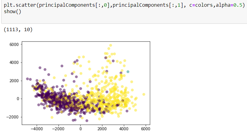
Data reconstruction
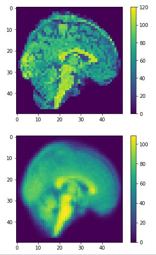
dim=50
approximation = pca.inverse_transform(principalComponents)
restored = approximation.reshape(-1,dim,dim,dim)
(1113, 50,50,50)
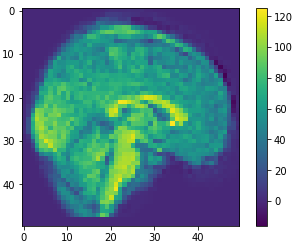
10
100
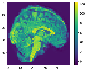
500
0.41
0.81
0.59
Eigen brains
- What is an Eigen brain
- Applying PCA
- Plotting
EigenBrains??
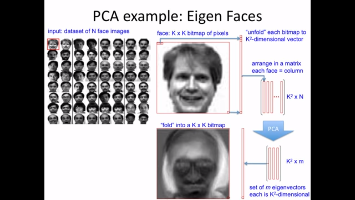

Applying PCA
1113x125000
125000x1113
125000x809
Transpose
PCA(99.9)
Reshaping

125000x809
Transpose
Reshape
50x50x50


eigen brain 809
eigen brain 1
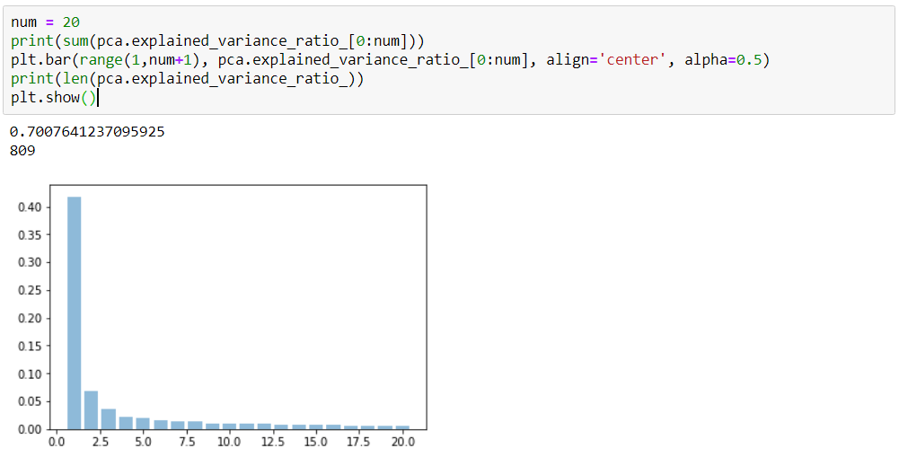
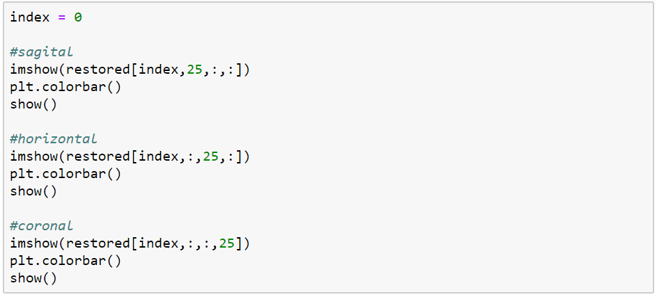
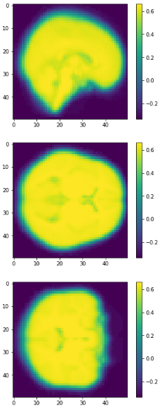
Plotting
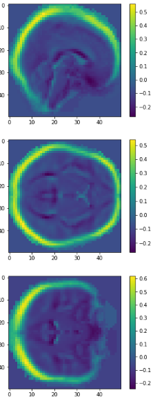
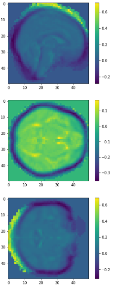

0.417
0.069
0.035
0.022
1
2
3
4
Separate classes
class1 = frame[(frame['class']== 1)]
print("Total class 1:", len(class1))
class2 = frame[(frame['class']== 0)]
print("Total class 0:", len(class2))
Total class 1: 550
Total class 0: 558
Average brains
from sklearn.preprocessing import normalize

average_brain1 = normalize(class1).mean(0)
average_brain2 = normalize(class2).mean(0)
avg_vol1 = average_brain1.reshape(50,50,50)
print(avg_vol1.shape)
avg_vol2 = average_brain2.reshape(50,50,50)
print(avg_vol2.shape)
(50, 50, 50)
(50, 50, 50)
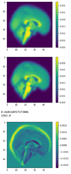
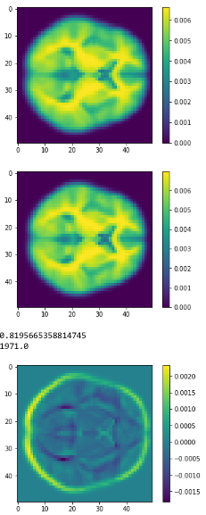
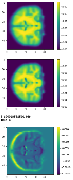
c1
c2
diff
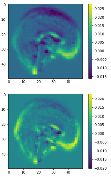

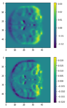
class1
class2
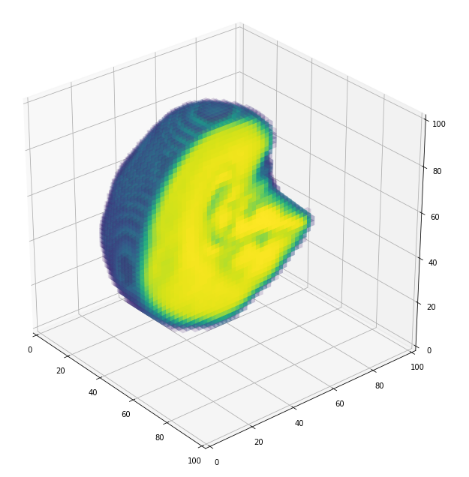
3D volume (fail)
jupyter notebook
PCA , Eigen brains
Classification
- Data pre-processing
- a bit more about the data.
- Resampling and hyperparameter tunning
- cross validation
- testing with different parameter values
- Models fittings
- underfitting and overfitting
- convergence
Post-PCA Data Proprocessing
After PCA:
- Data set of dimension 1113x1062 ('PCA.npy')
- Data in the form of array (npy format)
Clasification
- Data label of dimension 1113x1 ('Y.npy')
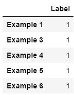
- Label 1 represents positive brains
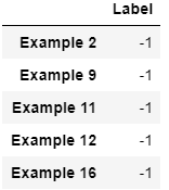
- Label -1 represent negative brains
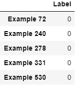
- Label 0 represent unlabeled brains
Post-PCA Data Proprocessing
Post-PCA Data Proprocessing
-Store the index of unlabeled examples & Remove them from the data set
-Replace examples of label -1 with 0 for classification training process (it is better to change to dummy label 0 and 1)
-Concatenate data set with the corresponding labels, rename the columns as PCA1, PCA2,....,PCA1062,CLASS
Post-PCA Data Proprocessing After PCA: Data set of dimension 1113x1062 ('PCA.npy') Data in the form of array (npy format) Clasification


Post-PCA Data Proprocessing
- Data label of dimension 1113x1 ('Y.npy')
- Label 1 represents positive brains
- Label -1 represent negative brains
- Label 0 represent unlabeled brains
Cleaning data
- Remove unlabeled data
- Change labels
- Concatenate data vs labels
- Evenly distribute data
Load Data & label data
(Remove unlabeled samples from the data set)
data=pd.DataFrame(np.load('PCA.npy'))
y=np.load('Y.npy')
y=pd.DataFrame(y)
dataset=pd.concat([data,y],axis=1)
index_remove=list(y[y[0]==0].index)
print(index_remove)
dataset=dataset.drop(index_remove)
[71, 239, 277, 330, 529]
Cleaning data
Replace examples of label -1 with 0 for classification training process (it is better to change to dummy label 0 and 1)
dataset['class'].replace(-1,0,inplace=True)


Cleaning data
Change labels
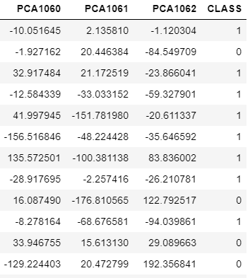
Rename the columns as PCA1, PCA2,....,PCA1062,CLASS
a=['PCA' + str(i+1) for i in range(1063)]
a[-1]='CLASS'
dataset.columns=a
Cleaning data
Evenly distribute data
Problem: Dataset is organized by example labels
class1 = dataset[(dataset['CLASS']== 1)]
print("Total class 1:", len(class1))
class0 = dataset[(dataset['CLASS']== 0)]
print("Total class 0:", len(class0))
df = []
for i in range(550):
df.append(class1.iloc[i].values)
df.append(class0.iloc[i].values)
for j in range(550,558):
df.append(class0.iloc[i].values)


class1 = dataset[(dataset['class']== 1)]
class2 = dataset[(dataset['class']== 0)]

Final processed data
np.save('X_y.npy',df)
- Save the processed data in .npy
- Load the final data
data=pd.DataFrame(np.load('X_y.npy'))
data.iloc[:,-1]=data.iloc[:,-1].apply(lambda i: int(i))
- Assign value to independent and dependent variables
y=np.array(data.iloc[:,-1].replace(-1,0)).ravel()
X=np.array(data.iloc[:,:-1])
Resampling Methods
The process of repeatedly drawing samples from data and refitting a given model on each sample
Resampling methods help:
- Learn more about the fitted model
- Estimates more accurately the error or accuracy for future data
- Estimates the bias and standard deviation of the hypothesized parameters
- Avoids over-fitting
But:
- Computationally expensive
- Underestimate or overestimate the real error
Resampling Methods
Techniques:
- Cross Validation
+ Validation set
+ Leave-one-out cross-validation (LOOCV)
+ K-fold cross validation
-
The Bootstrap
Resampling Methods
Validation Set
- Training data (70%): fitting purpose
- Validation set (20%): how good is the model for future data
- Test set (10%): generalization
train_percentage = 0.7
validation_percentage = 0.2
test_percentage = 0.1
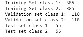
1108 examples
Resampling Methods
Validation Set
Problem: High bias and variability in error/accuracy between the splits.
E.g. For Support Vector Machine using Linear Kernel
Random split 1:
Random plit 2:
Random split 3:


The result highly dependent on 1 split is potentially biased
Resampling Methods
Leave-one-out cross-validation (LOOCV)
Leave-one-out cross-validation withholds only a single observation for the validation set.
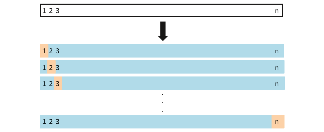
Okay, for our data set, at least 1103 times the model is fit!!!
Resampling Methods
K-fold cross validation
- The technique that randomly divides the whole data set into k subsets, groups or folds (k can be freely chosen)
- Each of k folds can be used as test set while other k-1 folds as training set.
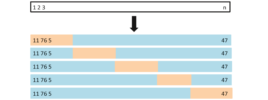
Resampling Methods
K-fold cross validation
Advantage:
- Less computationally expensive
- More accurate estimation for future data
- Easy to apply
- Applicable to large data
Disadvantage:
- Prone to underestimation of real error/overestimation of accuracy
- Not really effective for small data set
K-fold cross validation
from sklearn.model_selection import KFold
kf = KFold(n_splits=5)
kf.get_n_splits(X)

for train_index, test_index in kf.split(X): train_index
test_index


K-fold cross validation
Assign train_index,test_index to form
- X_train, y_train
- X_test, y_test
for train_index, test_index in kf.split(X):
X_train, X_test = X[train_index], X[test_index]
y_train, y_test = y[train_index], y[test_index]
Model fittings
- Logistic Regression using Regularization method (Ridge regression)
- Support Vector Machine with Linear Kernel
- Support Vector Machine with Gaussian Kernel
- K-nearest neighbors (k-nn)
- Neural Network
Model fittings
Problems: Over-fitting vs Under-fitting
Bias:
- how closeness is our predictive model’s to training data
- very little attention to the training data and oversimplifies the model
=>high error on training and test data
Variance:
- variability of model prediction for a given data point or a value showing spread of our data
- a lot of attention to training data and does not generalize on new data
=> perform very well on training data but badly on test data
Model fittings
Underfitting happens when a model unable to capture the underlying pattern of the data => high bias, low variance
Overfitting happens when model captures the noise along with the underlying pattern in data. In other words, our model is trained a lot over noisy data => low bias, high variance
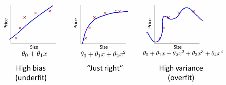
Model fittings
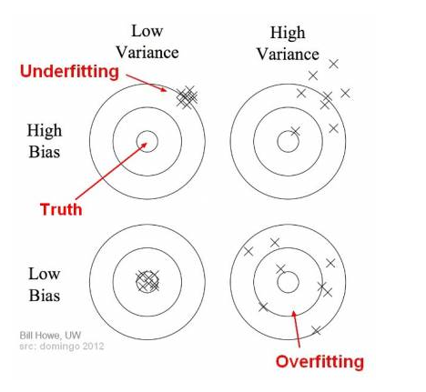
Why over-fitting:
- Too complex models, too many features
- Too small training data set
- Too small regularization term
...
Why under-fitting:
- Too simple model while the data are too complex
- Too large regularization term
Model fittings
Logistic Regression
- Also called Sigmoid Function
- In classification problem, the models should better output the prediction values over (0,1) => no sense for predicted values > 1 or < 0
E.g. 0 as non-spam email
1 as spam email
- Sometimes, linear regression does not work well (classification is not actually a linear function)
=> binary classification problem
Logistic Regression
Apply Sigmoid or Logistic Function

where:

Hypothesis or predicted output:

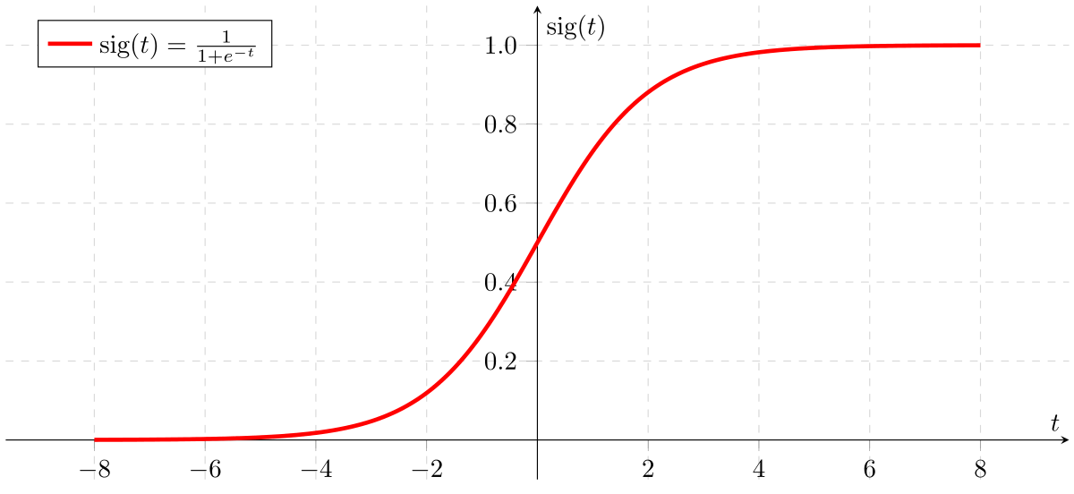

Logistic Regression
Cost function
To address overfitting as our dataset includes up to 1062 features
=> L1 Regularization term added
Logistic Regression using Regularization (Ridge regression)

Note:
Too large lambda could lead to under-fitting
Too small lambda could keep the model still over-fitting
Logistic Regression
Apply Logistic Regression
from sklearn.linear_model import LogisticRegression
def log_reg(X_train,X_test,y_train,y_test,reg_term):
classifier = LogisticRegression(solver='liblinear',penalty='l1',C=(1/reg_term),fit_intercept=True,max_iter=500)
classifier.fit(X_train,y_train)
return classifier.score(X_train,y_train),classifier.score(X_test,y_test)
Return the accuracy rate of the model over training and test set
Note:
C=1/(regularization term)
Logistic Regression
Define the best regularization term "lambda" for logistic regression model using cross validation
Number of folds: k=5
kf = KFold(n_splits=5)
List of regularization term :
param_logreg=[0.001*10**i for i in range(10)]

Logistic Regression
Step 1: find the best range with the best performance over both training and test set
training_acc_col=[]
test_acc_col=[]
for train_index, test_index in kf.split(X):
training_acc_col.append([])
test_acc_col.append([])
X_train, X_test = X[train_index], X[test_index]
y_train, y_test = y[train_index], y[test_index]
for i in param_logreg:
training_acc,test_acc=log_reg(X_train,X_test,y_train,y_test,i)
training_acc_col[-1].append(training_acc)
test_acc_col[-1].append(test_acc)
Logistic Regression
Plot averaged training accuracy & test accuracy over the range of regularization terms after running through 5 folds
x_i=[i for i in range(len(param_logreg))]
plt.figure(figsize=(10,10))
plt.plot(x_i,avg_training_acc,marker='o',mfc='blue',color='r')
plt.plot(x_i,avg_test_acc,marker='X',mfc='red',color='black')
plt.xticks(x_i,param_logreg)
plt.legend(['Training Accuracy','Test Accuracy'])
plt.xlabel('The Value of Regularization Terms',size=20)
plt.ylabel('Accuracy Rate',size=20)
plt.show()
avg_training_acc=np.mean(np.array(training_acc_col),axis=0)
avg_test_acc=np.mean(np.array(test_acc_col),axis=0)
Logistic Regression
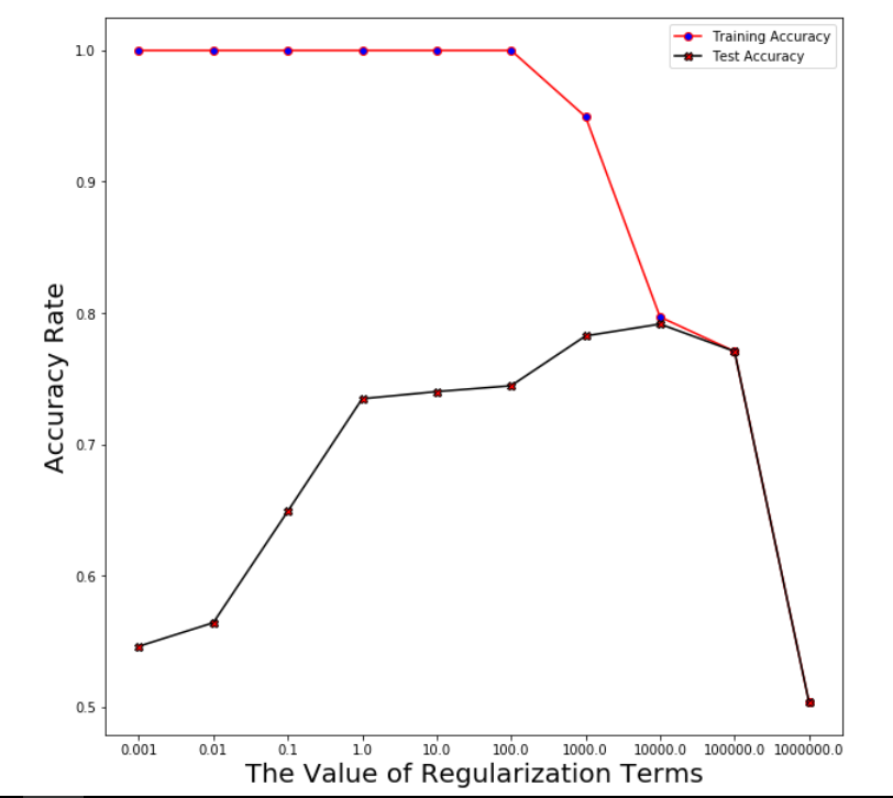
Logistic Regression
Step 2: Find the exact value of the best regularization term (we choose from 1000 to 10000)
param_logreg=[]
training_acc_col=[]
test_acc_col=[]
for i in range(1000,10000,500):
param_logreg.append(i)
for train_index, test_index in kf.split(X):
training_acc_col.append([])
test_acc_col.append([])
X_train, X_test = X[train_index], X[test_index]
y_train, y_test = y[train_index], y[test_index]
for i in param_logreg:
training_acc,test_acc=log_reg(X_train,X_test,y_train,y_test,i)
training_acc_col[-1].append(training_acc)
test_acc_col[-1].append(test_acc)
Logistic Regression
Plotting the averaged accuracy
avg_training_acc=np.mean(np.array(training_acc_col),axis=0)
avg_test_acc=np.mean(np.array(test_acc_col),axis=0)
x_i=[i for i in range(len(param_logreg))]
plt.figure(figsize=(10,10))
plt.plot(x_i,avg_training_acc,marker='o',mfc='blue',color='r')
plt.plot(x_i,avg_test_acc,marker='X',mfc='red',color='black')
plt.xticks(x_i,param_logreg)
plt.xlabel('The Value of Regularization Terms',size=20)
plt.ylabel('Accuracy Rate',size=20)
plt.legend(['Training Accuracy','Test Accuracy'])
# plt.xlim(min(param_logreg)/10,max(param_logreg))
plt.show()
Logistic Regression
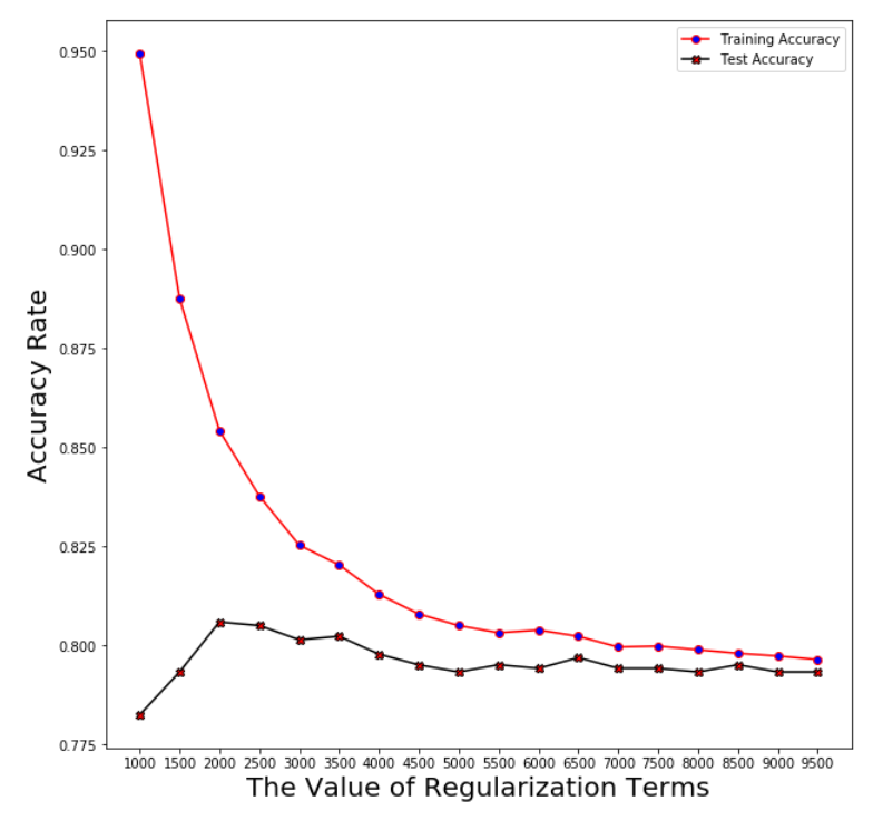
Logistic Regression
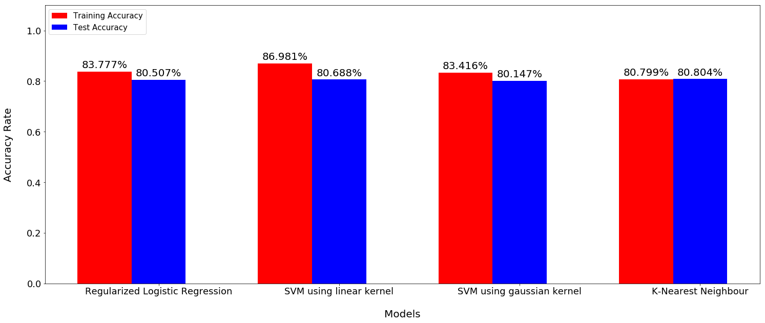
Regularization term: log_reg_term=2500
Averaged training accuracy: 83.78%
Averaged test accuracy: 80.51%
Support Vector Machine
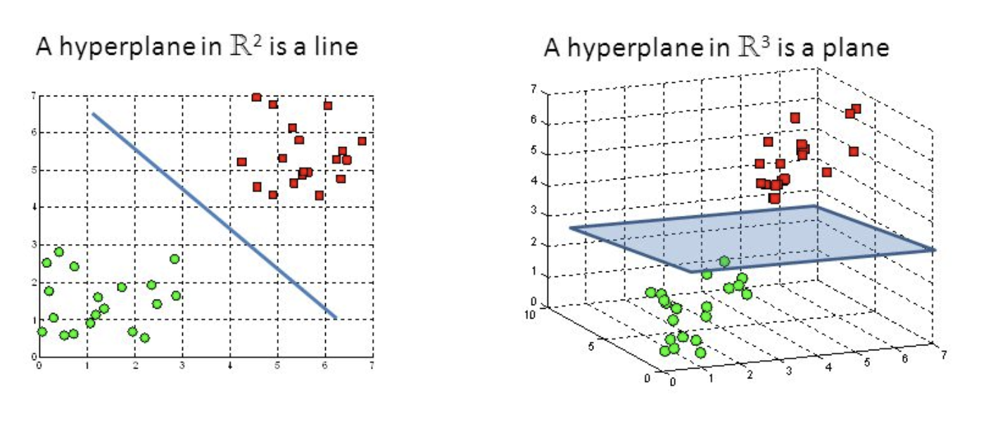
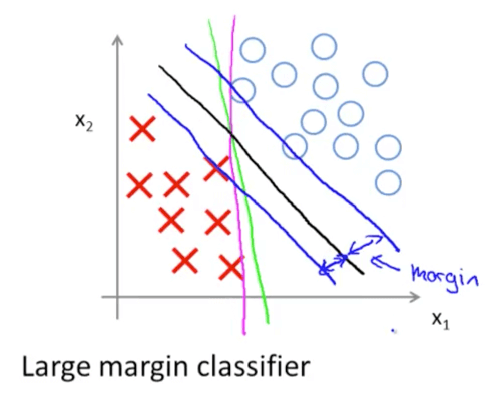
- A discriminative classifier formally defined by a separating hyperplane
- The algorithm outputs an optimal hyperplane which categorizes new examples (a line in 2-D dimension)
Support Vector Machine
Support Vector Machine

Cost Function

Objective Function
If C=(1/lambda), SVM with linear kernel and Logistic Regression using regularization give exactly the same hypothesized parameters
C too large: over-fitting
C too small: under-fitting
Instead of A + λB, we use CA + B
Support Vector Machine
kf = KFold(n_splits=5)
Applying Support Vector Machine with Linear Kernel
Number of folds (iterations): k=5
List of regularization terms:

=> Define the best regularization term
Support Vector Machine
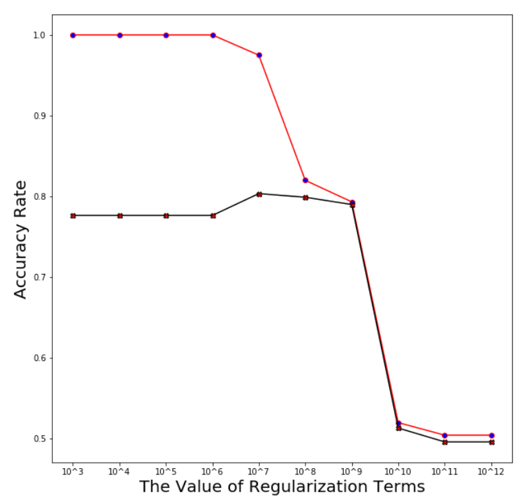
Define the best range of regularization terms
training_acc_col=[]
test_acc_col=[]
for train_index, test_index in kf.split(X):
training_acc_col.append([])
test_acc_col.append([])
X_train, X_test = X[train_index], X[test_index]
y_train, y_test = y[train_index], y[test_index]
for i in param_linear_svc:
training_acc,test_acc=linear_svc(X_train,X_test,y_train,y_test,i)
training_acc_col[-1].append(training_acc)
test_acc_col[-1].append(test_acc)
Support Vector Machine
Plotting the averaged training and test error after running through 5 folds
avg_training_acc=np.mean(np.array(training_acc_col),axis=0)
avg_test_acc=np.mean(np.array(test_acc_col),axis=0)
x_i=[i for i in range(len(param_linear_svc))]
plt.figure(figsize=(10,10))
ax = plt.subplot(111)
plt.plot(x_i,avg_training_acc,marker='o',mfc='blue',color='r')
plt.plot(x_i,avg_test_acc,marker='X',mfc='red',color='black')
xlabel=['10^'+str(i) for i in range(3,13)]
plt.xticks(x_i,xlabel)
plt.xlabel('The Value of Regularization Terms',size=20)
plt.ylabel('Accuracy Rate',size=20)
plt.show()
Support Vector Machine
Support Vector Machine
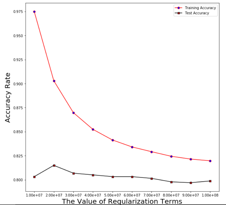
Find the exact value of the best regularization term (we choose from C = 10^7 to 10^8)
training_acc_col=[]
test_acc_col=[]
param_linear_svc=[i for i in range(10**7,10**8+1,int((10**7)))]
print('Regularization terms:',param_linear_svc)
for train_index, test_index in kf.split(X):
training_acc_col.append([])
test_acc_col.append([])
X_train, X_test = X[train_index], X[test_index]
y_train, y_test = y[train_index], y[test_index]
for i in param_linear_svc:
training_acc,test_acc=linear_svc(X_train,X_test,y_train,y_test,i)
training_acc_col[-1].append(training_acc)
test_acc_col[-1].append(test_acc)
Support Vector Machine
Plotting the averaged training and test error after running through 5 folds
Support Vector Machine
Regularization linear_svc_reg=3*10**7
Averaged training accuracy: 86.98%
Averaged test accuracy: 80.69%
Support Vector Machine
with Gaussian Kernel
Gaussian kernel a function whose value depends on the distance from the origin or from some point.
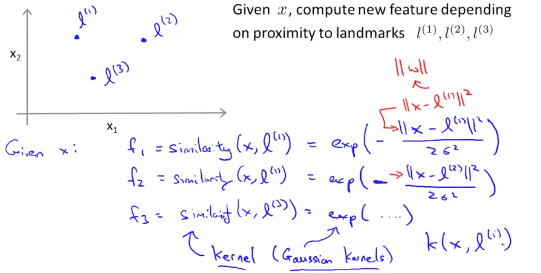
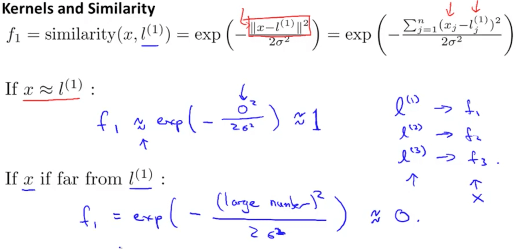
Support Vector Machine with Gaussian Kernel
Support Vector Machine with Gaussian Kernel
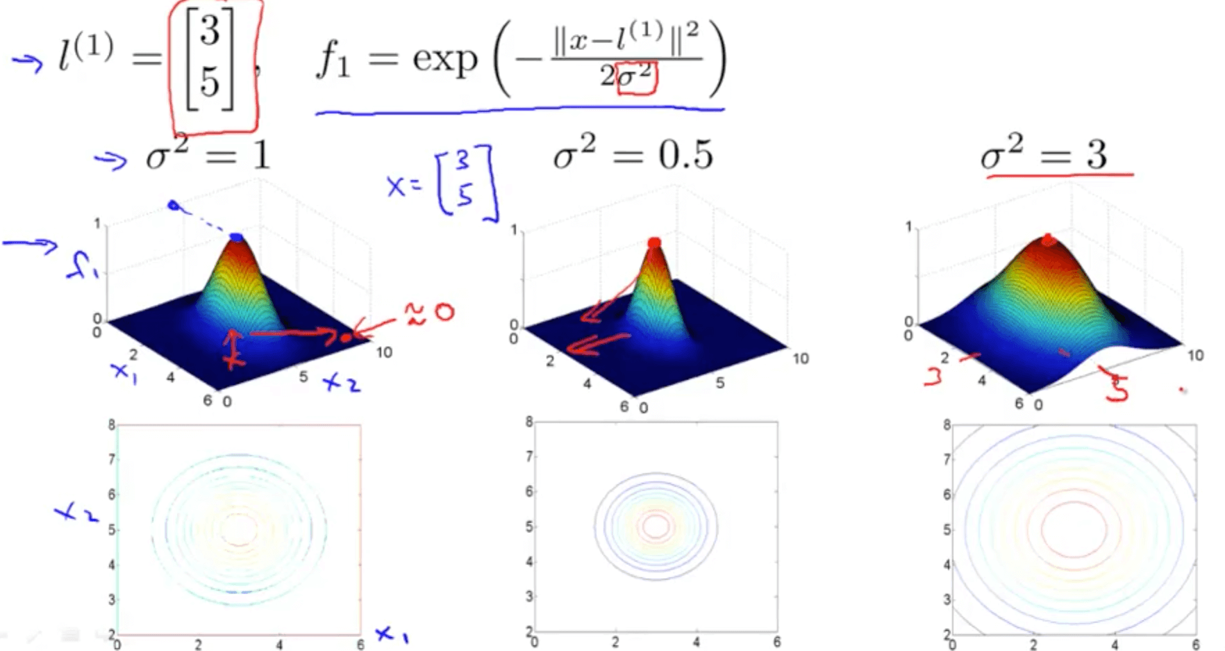
Defines how far the influence of a single training example reaches, with low values meaning ‘far’ and high values meaning ‘close’
E.g. Small sigma: small variance, 2 points must be so close to be defined as similar
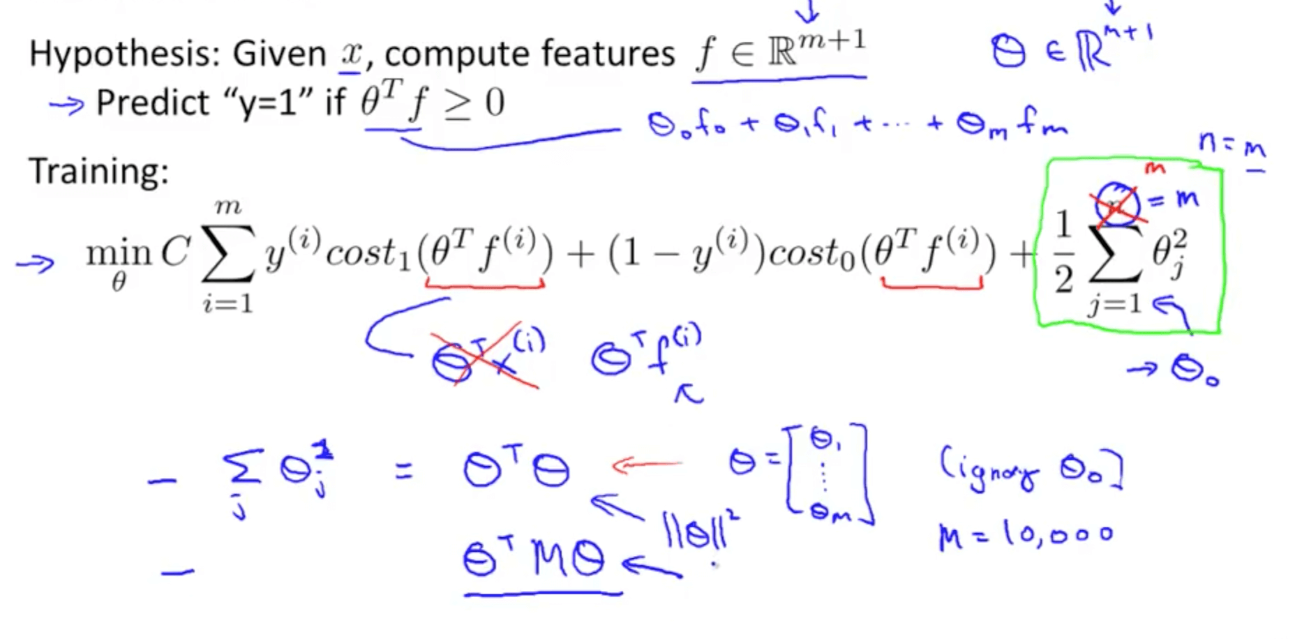
Support Vector Machine with Gaussian Kernel
Support Vector Machine with Gaussian Kernel
Applying Support Vector Machine with Gaussian Kernel
Number of folds (iterations): k=5
kf = KFold(n_splits=5)
List of regularization terms:
Regularization terms: Regs= [1, 10, 100, 1000]
Gammas= [10000, 100000, 1000000, 10000000, 100000000, 1000000000]
=> Define the best regularization term
Support Vector Machine with Gaussian Kernel
training_acc_col=[]
test_acc_col=[]
for train_index, test_index in kf.split(X):
print('FOLD:',k)
X_train, X_test = X[train_index], X[test_index]
y_train, y_test = y[train_index], y[test_index]
for i in reg_gaussian_svc:
training_acc_col.append([])
test_acc_col.append([])
for j in gamma_gaussian_svc:
print(j)
training_acc,test_acc=
gaussian_svc(X_train,X_test,y_train,y_test,i,j)
training_acc_col[-1].append(training_acc)
test_acc_col[-1].append(test_acc)
Support Vector Machine with Gaussian Kernel
avg_training_acc=np.mean(np.array(training_acc_col).reshape((5,-1)),axis=0).reshape(4,6)
avg_test_acc=np.mean(np.array(test_acc_col).reshape((5,-1)),axis=0).reshape(4,6)
Plotting the averaged training and test error after running through 5 folds
reg_gaussian_svc_i,gamma_gaussian_svc_i=np.meshgrid(np.array(reg_gaussian_svc),np.array(gamma_gaussian_svc),indexing='ij')
x_i=[i for i in range(len(reg_gaussian_svc))]
y_i=[i for i in range(len(gamma_gaussian_svc))]
x_ii,y_ii=np.meshgrid(x_i,y_i,indexing='ij')
plt.figure(figsize=(10,10))
plt.contourf(x_ii,y_ii,avg_training_acc)
plt.colorbar()
plt.xticks(x_i,reg_gaussian_svc)
plt.yticks(y_i,gamma_gaussian_svc)
plt.show()
plt.figure(figsize=(10,10))
plt.contourf(x_ii,y_ii,avg_test_acc)
plt.colorbar()
plt.xticks(x_i,reg_gaussian_svc)
plt.yticks(y_i,gamma_gaussian_svc)
plt.show()
Support Vector Machine with Gaussian Kernel

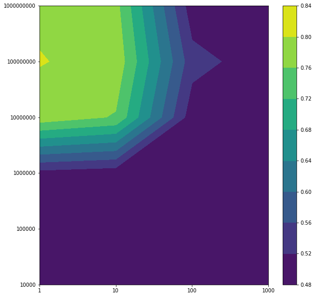
Support Vector Machine with Gaussian Kernel
best_reg=0
best_gamma=0
training_acc_col=[]
test_acc_col=[]
for train_index, test_index in kf.split(X):
X_train, X_test = X[train_index], X[test_index]
y_train, y_test = y[train_index], y[test_index]
for i in reg_gaussian_svc:
for j in gamma_gaussian_svc:
training_acc,test_acc=
gaussian_svc(X_train,X_test,y_train,y_test,i,j)
test_acc_col.append(test_acc)
avg_test_acc=np.mean(np.array(test_acc_col).reshape((5,-1)),axis=0).reshape(4,6)
best_test_accuracy=np.max(avg_test_acc)
i,j=int(np.where(avg_test_acc==np.max(avg_test_acc))[0]),int(np.where(avg_test_acc==np.max(avg_test_acc))[1])
best_reg=reg_gaussian_svc[i]
best_gamma=gamma_gaussian_svc[j]
Support Vector Machine with Gaussian Kernel
Support Vector Machine with Gaussian Kernel
Regularization terms: Regs= [1, 10, 100, 1000]
Gammas= [10000, 100000, 1000000, 10000000, 100000000, 1000000000]

Best test accuracy: 0.8014716073539603
Best regularization term: 1
Best gamma: 100000000
K nearest neighbors
(KNN)
the input consists of the k closest training examples in the feature space.
(modified pipeline)
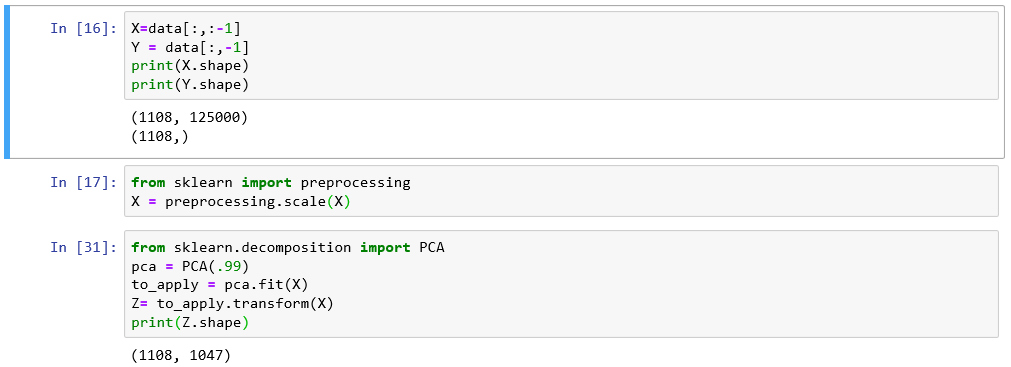
PCA should only be applied on the training set
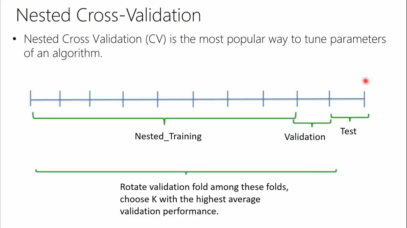
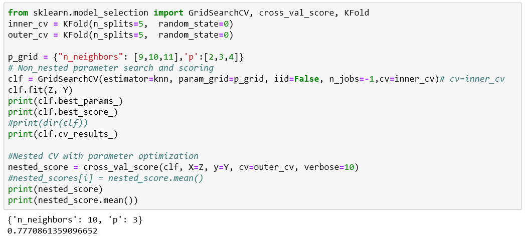
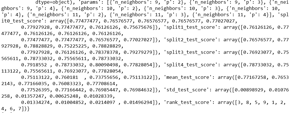
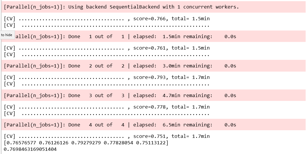
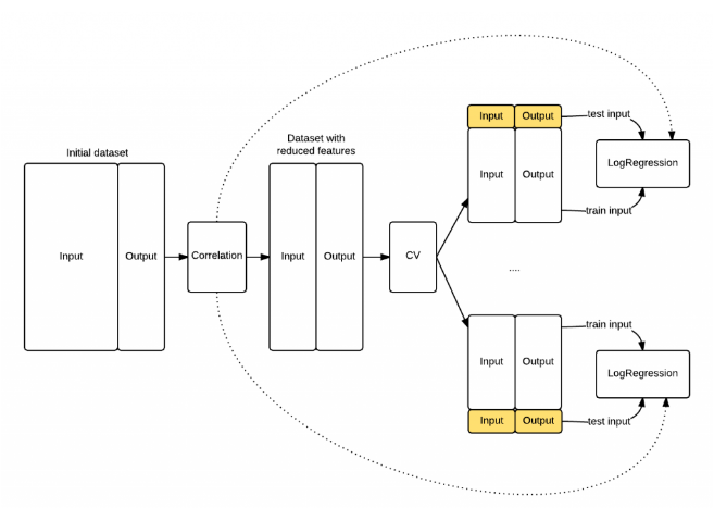
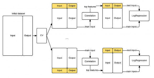
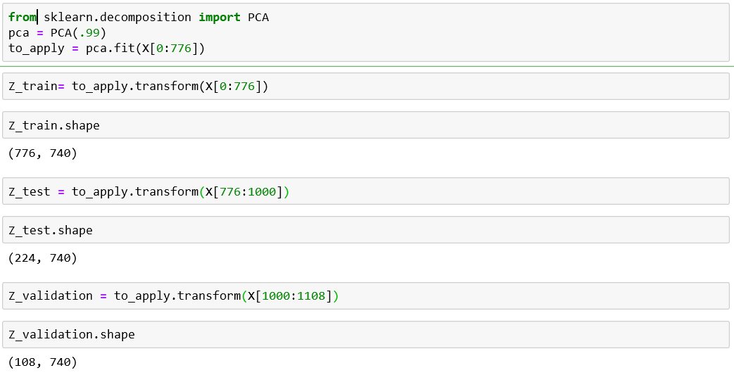
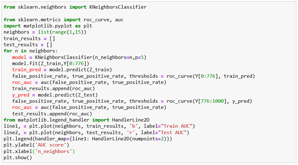
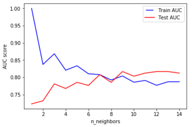

best parameters only for that test fold!!!
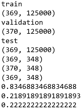
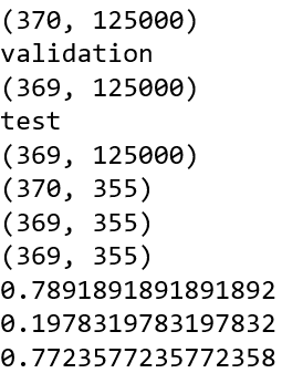
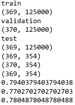
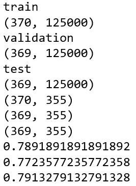
Model Performance
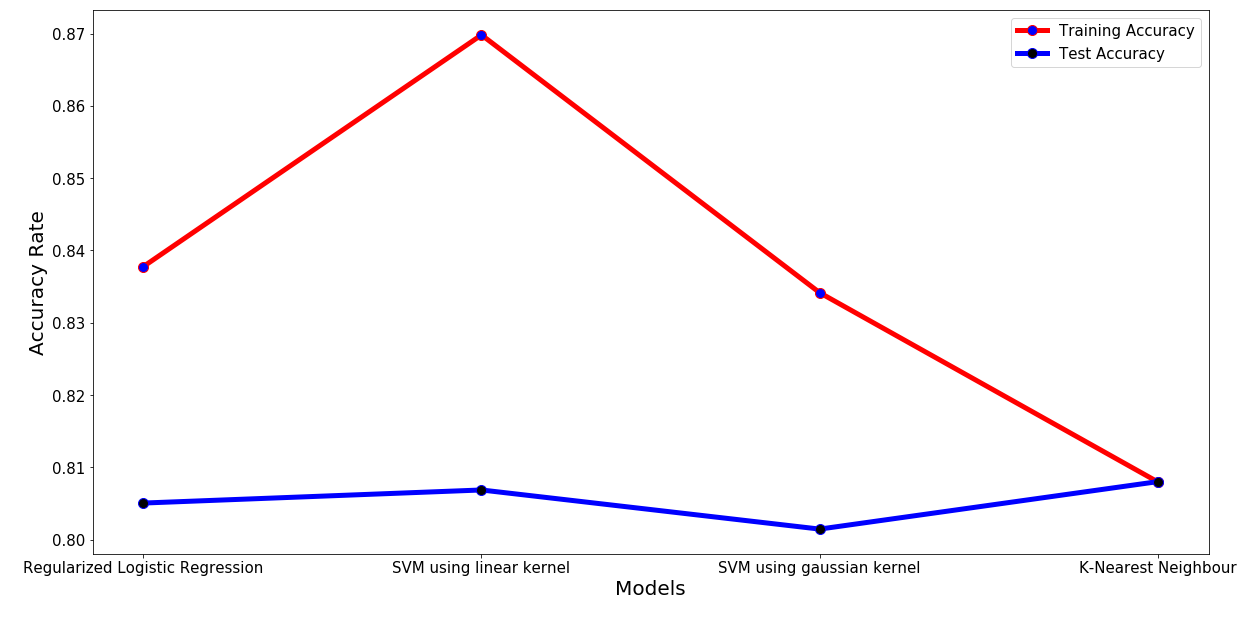
Model Performance
PCA applied to generated folds
PCA + Nested cross-validation
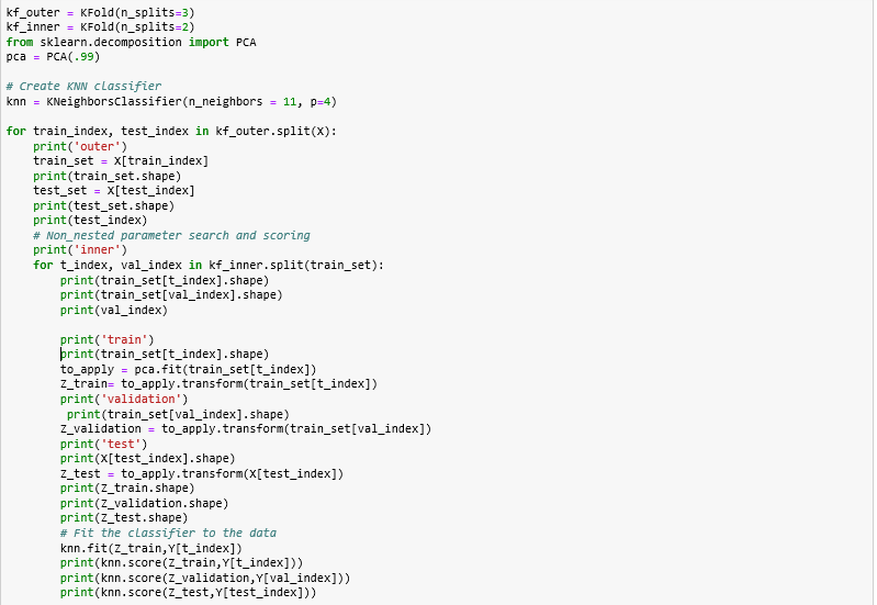
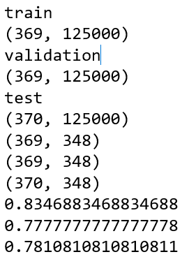
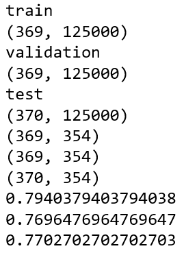
???
[1108x155x165x195x1]


1108
1


[256x256x256]
[155x165x195]
Original
Cropped


Input Tensor
Layer (type) Output Shape Param #
=================================================================
conv1 (Conv3D) (None, 155, 165, 195, 8) 1728008
_________________________________________________________________
max_pooling3d (MaxPooling3D) (None, 51, 55, 65, 8) 0
_________________________________________________________________
conv2 (Conv3D) (None, 51, 55, 65, 16) 2000016
_________________________________________________________________
max_pooling3d_1 (MaxPooling3 (None, 25, 27, 32, 16) 0
_________________________________________________________________
conv3 (Conv3D) (None, 25, 27, 32, 32) 1728032
_________________________________________________________________
max_pooling3d_2 (MaxPooling3 (None, 12, 13, 16, 32) 0
_________________________________________________________________
conv3d (Conv3D) (None, 12, 13, 16, 64) 2048064
_________________________________________________________________
max_pooling3d_3 (MaxPooling3 (None, 6, 6, 8, 64) 0
_________________________________________________________________
conv3d_1 (Conv3D) (None, 6, 6, 8, 128) 1024128
_________________________________________________________________
max_pooling3d_4 (MaxPooling3 (None, 3, 3, 4, 128) 0
_________________________________________________________________
flatten (Flatten) (None, 4608) 0
_________________________________________________________________
dense (Dense) (None, 2048) 9439232
_________________________________________________________________
dense_1 (Dense) (None, 512) 1049088
_________________________________________________________________
predictions (Dense) (None, 1) 513
=================================================================
Total params: 19,017,081
Trainable params: 19,017,081
Non-trainable params: 0
[1108] [X^3]


1108
1


[256x256x256]
[200^3]
Original
Cropped


Input Tensor


[150^3, 100^3, 50^3]
Resized
Conclusions
- It is possible to reduce the dimension using simple operations like: cropping and resizing , however, this also means we lose information.
- Aspect ratio in not conserved during resize step (warping)
- PCA help us reduce the amount of features by finding a subspace in which classes can be seperated normally using the principal components as new axes for our data.
- PCA can be used for different purposes depending the application.
- The computation of PCA is fairly expensive and can be speeded up by using SVD algorithm.
- Vizualization of volumes is expensive...(GPU based solutions)
- Feature selection should be applied ONLY to the train data BEFORE cross validation step.
- Nested cross validation is needed in order to eliminate the bias coming from parameter search (learning only for a piece of data).
- PCA should be applied with care due to introdution of bias if done wrong (leak of knowledge)
- Nestes cross validation is computational expensive due to inner and outer loops (parameter search + cross val)
- Work with cropped 3D volumes in future developments 5million voxels instead of 17million (convolutional neural networks starting point)