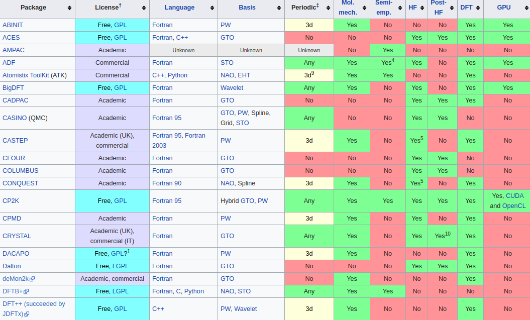
Computational Studies of Electron Systems

\displaystyle \int\limits_0^\infty

int main()
{
    printf("Hello world\n");
    return 0;
}

\textrm{d}t=\textrm{DFT}

Gergő Kukucska

september, 2018

Single body problem

\hat{H}|\psi\rangle=E|\psi\rangle

\hat{H}=\hat{T}+\hat{V}

\hat{T}=\frac{-\hbar^2\nabla^2}{2m}\quad\hat{V}=V(\mathbf{r})

Analytically solvable for numerous cases:

Harmonic oscillator
Hydrogen atom
etc....

Two body problem

\hat{H}|\psi\rangle=E|\psi\rangle

\hat{H}=\hat{T}+\hat{V}+\hat{W}

\hat{T}=\frac{-\hbar^2\nabla_1^2}{2m}+\frac{-\hbar^2\nabla_2^2}{2m}

\hat{V}=V(\mathbf{r}_1)+V(\mathbf{r}_2)\quad \hat{W}=V_{ee}(\mathbf{r}_1-\mathbf{r}_2)

Scattering problem:

Born approximation
Partial waves

Helium atom: 1 nucleus and 2 electrons

\hat{H}=\frac{-\hbar^2\nabla_1^2}{2m}+\frac{-\hbar^2\nabla_2^2}{2m}+\frac{-\hbar^2\nabla_I^2}{2M}+\hat{W}

\hat{W}=V_{ee}(\mathbf{r}_1-\mathbf{r}_2)+V_{en}(\mathbf{R}_I-\mathbf{r}_1)+V_{en}(\mathbf{R}_I-\mathbf{r}_2)

Born-Oppenheim approximation: \(m<<M\)

\Psi(\lbrace R_I\rbrace,\lbrace r_i\rbrace)=\Phi(\lbrace R_I\rbrace)\cdot \psi(\lbrace R_I\rbrace,\lbrace r_i\rbrace)

Helium atom: 1 nucleus and 2 electrons

\hat{H}=\frac{-\hbar^2\nabla_1^2}{2m}+\frac{-\hbar^2\nabla_2^2}{2m}+\frac{-\hbar^2\nabla_I^2}{2M}+\hat{W}

\hat{W}=V_{ee}(\mathbf{r}_1-\mathbf{r}_2)+V_{en}(\mathbf{R}_I-\mathbf{r}_1)+V_{en}(\mathbf{R}_I-\mathbf{r}_2)

Born-Oppenheim approximation: fixed nuclei

Analytically unsolvable

\hat{H}=\underbrace{\frac{-\hbar^2\nabla_1^2}{2m}+V_{en}(\mathbf{R}_I-\mathbf{r}_1)}_{\textrm{Hydrogen-like}}+ \underbrace{\frac{-\hbar^2\nabla_2^2}{2m}+V_{en}(\mathbf{R}_I-\mathbf{r}_2)}_{\textrm{Hydrogen-like}}+\\ +V_{ee}(\mathbf{r}_1-\mathbf{r}_2)

Assimptotic methods:

perturbation: \(V_{ee}\) as small perturbation
- Problem: Huge first order corrections (many orders needed to converge), need description of scattering states
variation calculus:

E[\psi]=\frac{\langle\psi|\hat{H}|\psi\rangle}{\langle\psi|\psi\rangle}

\delta E=0 \leftrightarrow \hat{H}|\psi\rangle=E|\psi\rangle

Practical implementation:

\(|\psi\rangle\) ansatz is the function of some parameters \(\lbrace a_j\rbrace\)
- Anti-symmetric: \(\psi (1,2)=-\psi (2,1)\)
Calculating the regular \(E(a_j)\) function and minimizing it

best one Slater determinant solution: Hartree-Fock equations:

Who's got the largest.... ansatz?

More parameters \(\rightarrow\) larger parameterspace \(\rightarrow\) better \(E_0\)
Convenient ansatz: Slater-determinant

|\psi\rangle=\frac{1}{\sqrt{2}} \left| \begin{matrix} \psi_1(1)&\psi_1(2)\\ \psi_2(1)&\psi_2(2)\\ \end{matrix} \right| =\frac{\psi_1(1)\psi_2(2)-\psi_1(2)\psi_2(1)}{\sqrt{2}}

\displaystyle \hat{T}\psi_1(\mathbf{r}_1)+V_{en}(\mathbf{r}_1)\psi_1(\mathbf{r}_1)+ \underbrace{\int\textrm{d}\mathbf{r}_2V_{ee}(\mathbf{r}_1-\mathbf{r}_2)|\psi_2(\mathbf{r}_2)|^2\psi_1(\mathbf{r}_1)}_\textrm{Coulomb term}-\\- \underbrace{\int\textrm{d}\mathbf{r}_2V_{ee}(\mathbf{r}_1-\mathbf{r}_2)\psi^*_2(\mathbf{r}_2)\psi_1(\mathbf{r}_2)\psi_2(\mathbf{r}_1)}_\textrm{Exchange term}=E_{HF}\psi_1(\mathbf{r}_1)

\(E_{HF}\) is not the experimental energy
- What's better than a Slater determinant?
- Two Slater determinant
  - includes correlation effects

What does correlation mean?

Different types of correlation:

Radial correlation: electrons orbiting with different radius
Angular correlation: electrons avoiding to be on the same side of the nuclei: \(\psi\approx 0\) if \(\varphi_1\approx \varphi_2\), \(\theta_1\approx \theta_2\)
Coulomb hole: electrons completely avoid each other: \(\psi\approx 0\) if r\(_1\approx\) r\(_2\)
Fermi hole (larger atoms): result of Pauli's exclusion principle
- triplet spin state: \(|\uparrow\uparrow\rangle\)
  - anti symmetric spatial part \(\psi\approx 0\) if r\(_1\approx\) r\(_2\)
- singlet spin state:\(\displaystyle\frac{(|\downarrow\uparrow\rangle-|\uparrow\downarrow\rangle)}{\sqrt{2}}\)
  - symmetric spatial part \(\psi\neq 0\) if r\(_1\approx\) r\(_2\)

E_\textrm{exp}=E_\textrm{HF}+E_\textrm{c}

Brute force always works!

Completely numeric solution with finite element methods:

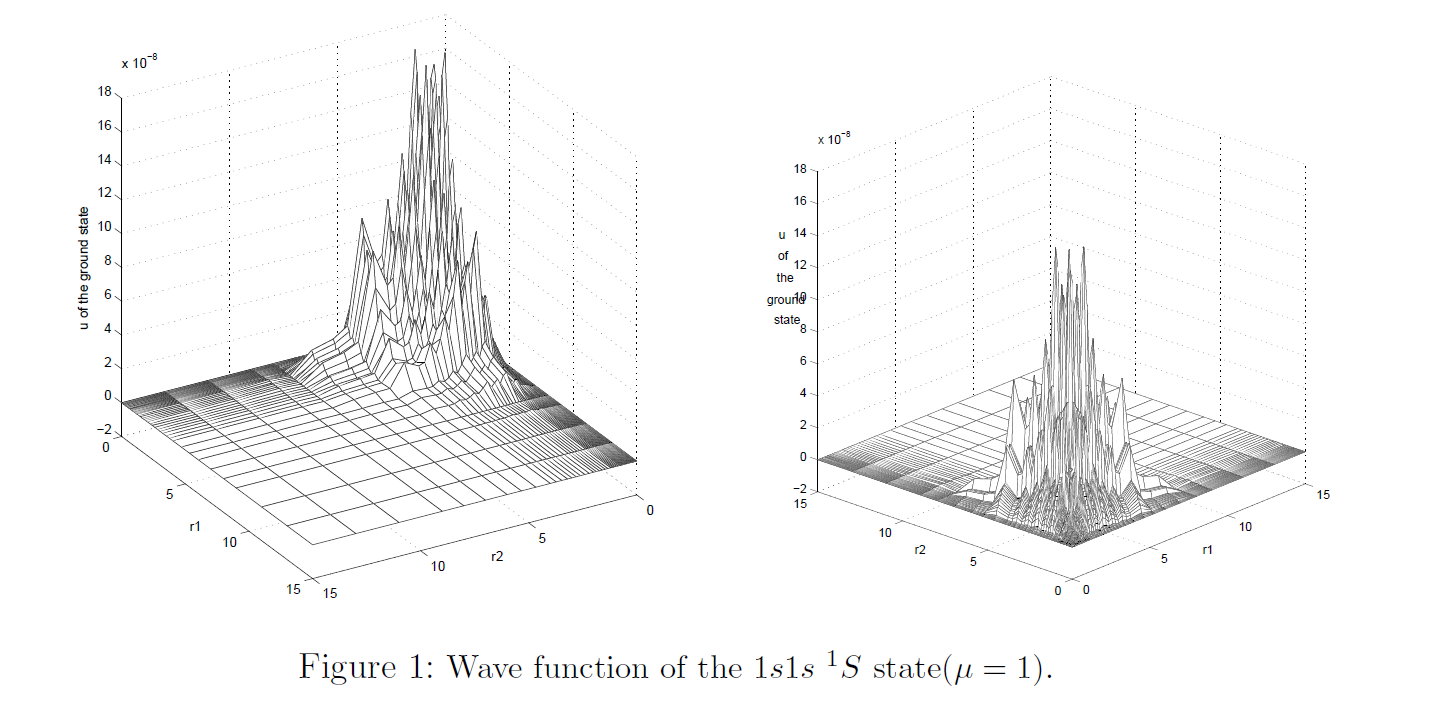
Zheng, W. and Ying, L. (2004), Int. J. Quantum Chem., 97: 659-669. doi:10.1002/qua.10770

End of the semester

for astrophysicists....

Many body problem

\hat{H}|\psi\rangle=E|\psi\rangle

\hat{H}=\hat{T}+\hat{V}+\hat{W}

\hat{T}=\sum\limits_{i=1}^{N_e}\frac{-\hbar^2\nabla_i^2}{2m}+ \sum\limits_{I=1}^{N_n}\frac{-\hbar^2\nabla_I^2}{2M_I}

\hat{V}=\sum\limits_{i,I}V_{en}(\mathbf{r}_i-\mathbf{R}_I)\\ \hat{W}=\frac{1}{2}\sum\limits_{i,j}V_{ee}(\mathbf{r}_i-\mathbf{r}_j)+\frac{1}{2}\sum\limits_{I,J}V_{nn}(\mathbf{R}_I-\mathbf{R}_J)

Many body problem

\left(\sum\limits_{i=1}^{N_e}\frac{-\hbar^2\nabla_i^2}{2m}+\sum\limits_{i,I}V_{en}(\mathbf{r}_i-\mathbf{R}_I)+\frac{1}{2}\sum\limits_{i,j}V_{ee}(\mathbf{r}_i-\mathbf{r}_j)+\right.\\ \left.+\frac{1}{2}\sum\limits_{I,J}V_{nn}(\mathbf{R}_I-\mathbf{R}_J)\right)\psi(\lbrace\mathbf{R}_I\rbrace,\lbrace\mathbf{r}_i\rbrace)=\\\left. =E_e(\lbrace\mathbf{R}_I\rbrace,\lbrace\mathbf{r}_i\rbrace)\psi(\lbrace\mathbf{R}_I\rbrace,\lbrace\mathbf{r}_i\rbrace)\right.

Born-Oppenheim approximation: \(m<<M\)

\Psi(\lbrace R_I\rbrace,\lbrace r_i\rbrace)=\Phi(\lbrace R_I\rbrace)\cdot \psi(\lbrace R_I\rbrace,\lbrace r_i\rbrace)

Separated Schrödinger equations:

\left(\sum\limits_{I=1}^{N_n}\frac{-\hbar^2\nabla_I^2}{2M_I}+E_e(\lbrace R_I\rbrace)\right)\Phi(\lbrace R_I\rbrace)=E(\lbrace R_I\rbrace)

Many body problem

Cross term:

\hat{B}=\sum\limits_I\hat{T}(I)\psi(\{\mathbf{r}_i\},\{\mathbf{R}_I\})

Two approximations:

Born-Oppenheimer approximation: \(\hat{B}\)=0
Adiabatic approximation: effect of \(\hat{B}\) as expectation value

When does it matter?

Only if the energy of two electronic states are close (conical intersection)
Slightly change the optimal configuration of atoms

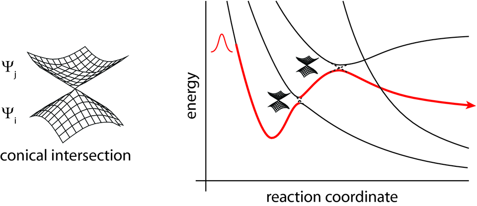
Conical intersection

Brute force always works?

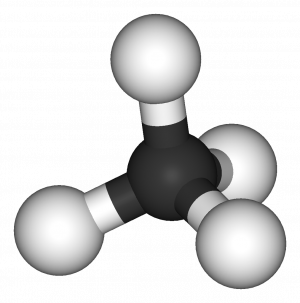
1 Carbon, 4 Hydrogen = 10 electrons

30 independent coordinates

(excluding spin)

100 point per coordinate

\(100^{30}=10^{60}\) Complex number

1Complex number /\( 1\textrm{\AA}^3 \) (Using spins as bits)

Wavefunction stored in ~\(10^{30}\,\textrm{m}^3\)

The world is not enough...Literally!!!!

Volume of earth:

\(4\pi/3\cdot(6.37)^3\cdot10^{18}\textrm{m}^3\approx10^{21}\textrm{m}^3\)

We need 1 billion earth!

<<\LARGE

We don't have 1 billion earths... YET!!!

Until we get enough storage... Let's think!

Apply symmetry considerations?

improvement by 2-100 factor

Reduce number of coordinates?

Consider only half of the independent coordinates

15 independent coordinates, 100 point per coordinate

\(100^{15}=10^{30}\) Complex number,1Complex number /\( 1\textrm{\AA}^3 \)

Wavefunction stored in ~\(10^{1}\,\textrm{m}^3\)

Only 10 box of wood is enough!

Hohenberg-Kohn theorems

We can reduce the number of coordinates to 3!

Consider an interacting many-body system in an external potential:

Hohenberg-Kohn I: The external potential (\(v_\textrm{ext}\)), and hence the total energy, is a unique functional of the electron density (\(n(\mathbf{r})\)).

Hohenberg-Kohn II: The groundstate energy can be obtained variationally: the density that minimises the total energy is the exact groundstate density.

Hohenberg-Kohn I: The external potential (\(v_\textrm{ext}\)), and hence the total energy, is a unique functional of the electron density (\(n(\mathbf{r})\)).

The usual way:

The external \(v_\textrm{ext}\) potential defines the Hamiltonian \(\hat{H}\)

\hat{H}|\psi\rangle=E|\psi\rangle

Ground state obatined by solving:

Electron density obtained:

\displaystyle n(\mathbf{r})=\int\prod\limits_{i=2}^{N_e}\textrm{d} \mathbf{r}_i |\psi(\mathbf{r},\mathbf{r}_2,\dots,\mathbf{r}_{N_e})|^2

What's new?

Hohenberg-Kohn I: The external potential (\(v_\textrm{ext}\)), and hence the total energy, is a unique functional of the electron density (\(n(\mathbf{r})\)).

The Hohenberg-Kohn way:

The external \(v_\textrm{ext}\) potential defines the Hamiltonian \(\hat{H}\)

\hat{H}|\psi\rangle=E|\psi\rangle

Ground state obatined by solving:

Electron density obtained:

\displaystyle n(\mathbf{r})=\int\prod\limits_{i=2}^N\textrm{d} \mathbf{r}_i |\psi(\mathbf{r},\mathbf{r}_2,\dots,\mathbf{r}_N)|^2

What's new?

THE RELATION IS UNIQUE AND REVERSIBLE!!!

Hohenberg-Kohn I: The external potential (\(v_\textrm{ext}\)), and hence the total energy, is a unique functional of the electron density (\(n(\mathbf{r})\)).

Lets prove it!

\hat{H_1}=\sum\limits_{i=1}^{N}\hat{T}(i)+\hat{W}_{ee}+\hat{V}_1\quad \hat{H_2}=\sum\limits_{i=1}^{N}\hat{T}(i)+\hat{W}_{ee}+\hat{V}_2

\hat{H_1}|\psi\rangle=E_1|\psi\rangle\qquad \hat{H_2}|\psi\rangle=E_2|\psi\rangle

(\hat{V}_1-\hat{V}_2)|\psi\rangle=(E_1-E_2)|\psi\rangle

\sum\limits_{i=1}^{3N}(v_1(\mathbf{r}_i)-v_2(\mathbf{r}_i))\psi(\mathbf{r}_1,\mathbf{r}_2,\dots,\mathbf{r}_N)=(E_1-E_2)\psi(\mathbf{r}_1,\mathbf{r}_2,\dots,\mathbf{r}_N)

This must be satisfied in all points, thus \(\hat{V}_1\)\(=\hat{V}_2+\) constant

\hat{V}_1\neq\hat{V}_2+\textrm{constant}

Round 1: Proove that two external potential can't yield the same ground state wavefunction

Hohenberg-Kohn I: The external potential (\(v_\textrm{ext}\)), and hence the total energy, is a unique functional of the electron density (\(n(\mathbf{r})\)).

Round 2: Prove that two different wavefunction cannot yield the same density

\hat{H_1}|\psi_1\rangle=E_1^0|\psi_1\rangle\quad \hat{H_2}|\psi_2\rangle=E_2^0|\psi_2\rangle

E_1^0=\langle\psi_1|\hat{H}_1|\psi_1\rangle<\langle\psi_2|\hat{H}_1|\psi_2\rangle=\langle\psi_2|\hat{H}_2|\psi_2\rangle+\langle\psi_2|\hat{V}_1-\hat{V}_2|\psi_2\rangle

\displaystyle E_1^0 < E_2^0+\int n_0(\mathbf{r})\lbrace v_1(\mathbf{r})-v_2(\mathbf{r})\rbrace

\displaystyle E_2^0 < E_1^0+\int n_0(\mathbf{r})\lbrace v_2(\mathbf{r})-v_1(\mathbf{r})\rbrace

\displaystyle E_2^0 +E_1^0< E_1^0+E_2^0

Hohenberg-Kohn II: The groundstate energy can be obtained variationally: the density that minimises the total energy is the exact groundstate density.

Already prooven relation:

\psi\Longleftrightarrow n(\mathbf{r}),\quad E[n(\mathbf{r})]

E[n(\mathbf{r})]=\langle\psi|\hat{H}|\psi\rangle+\langle\psi|\hat{V}_\textrm{ext}|\psi\rangle

Consider other \(|\psi'\rangle\) wavefunction:

E[n'(\mathbf{r})]=\langle\psi'|\hat{H}|\psi'\rangle+\langle\psi'|\hat{V}_\textrm{ext}|\psi'\rangle

From the variational principle:

\langle\psi'|\hat{H}|\psi'\rangle+\langle\psi'|\hat{V}_\textrm{ext}|\psi'\rangle> \langle\psi|\hat{H}|\psi\rangle+\langle\psi|\hat{V}_\textrm{ext}|\psi\rangle

E[n'(\mathbf{r})]>E[n(\mathbf{r})]

Next step?

Equality constrain!

\delta E[n(\mathbf{r})]=0

\displaystyle \int n(\mathbf{r})\textrm{d}\mathbf{r}=N_e

Modified functional:

\displaystyle \delta\left[E[n(\mathbf{r})]+\mu\left(N_e-\int n(\mathbf{r})\textrm{d}\mathbf{r}\right)+\int n(\mathbf{r})v_\textrm{ext}(\mathbf{r})\textrm{d}\mathbf{r}\right]=0

Two way to solve it:

Thomas-Fermi approximation
Kohn-Sham equation

Euler equation:

\displaystyle \frac{\delta E[n(\mathbf{r})]}{\delta n(\mathbf{r})} +v_\textrm{ext}(\mathbf{r})=\mu

Thomas-Fermi approximation

Kinetic part of \(E[n]\) from Heisenbergs uncertainity:

\Delta p_x \Delta x \geq h

V_{ph}=V_\textrm{real}V_\textrm{momentum}=V\frac{4\pi}{3}p_F^3(\mathbf{r})

Kinetic energy density:

Relation between maximal momentum and density:

Volume of the phase space:

Number of states within the phase space:

N=2V_{ph}/h^3=V\frac{8\pi}{3h^3}p_F^3(\mathbf{r})

p_F(\mathbf{r})=\left(\frac{3h^3}{8\pi}\right)^{1/3}n(\mathbf{r})^{1/3}

\displaystyle t=\frac{1}{V}\int\frac{p^2}{2m}\textrm{d}N=\int\limits_0^{p_F}\frac{p^2}{2m}\frac{4\pi p^2V\cdot 2}{h^3}\textrm{d}p=C_\textrm{kin}n(\mathbf{r})^{5/3}

Thomas-Fermi approximation

Total energy functional:

\displaystyle E[n]=\int\textrm{d}\mathbf{r}C_\text{kin}n^{5/3}(\mathbf{r})+V_\text{ext}(\mathbf{r})n(\mathbf{r})+\frac{1}{2}\int\textrm{d}\mathbf{r'}\frac{n(\mathbf{r})n(\mathbf{r}')}{|\mathbf{r}-\mathbf{r}'|}

Euler equation:

\displaystyle \frac{5}{3}C_\text{kin}n^{2/3}(\mathbf{r})+V_\text{ext}(\mathbf{r})+\int\textrm{d}\mathbf{r'}\frac{n(\mathbf{r}')}{|\mathbf{r}-\mathbf{r}'|}=\mu

Pros:

Self consistent description of quasi-classic electron system
Good for qualitative description of weekly interacting \(e^-\) gas

Cons:

Approximate kinetic energy
No exchange term
Can't describe strongly oscillating systems

Kohn-Sham equations

Search the wavefunction in a single Slater-determinant form:

\displaystyle \Phi=\frac{1}{N!}\textrm{det}(\varphi_1,\varphi_2,\dots,\varphi_{N_e})

Kinetic energy:

\displaystyle T=\sum\limits_i^{N_e}\int\text{d}\mathbf{r}\varphi_i^*(\mathbf{r})\frac{-\hbar^2\nabla^2}{2m}\varphi_i(\mathbf{r})

Self interaction energy:

\displaystyle W=\frac{1}{2}\int\text{d}\mathbf{r}\text{d}\mathbf{r}'\frac{n(\mathbf{r})n(\mathbf{r}')}{|\mathbf{r}-\mathbf{r}'|}+E_{xc}[n(\mathbf{r})]

\displaystyle \langle\hat{A}\rangle=\left\langle\sum\limits_i^{N_e}\hat{A}_i\right\rangle=\sum\limits_i^{N_e}\langle\varphi_i|\hat{A}_i|\varphi_i\rangle

Kohn-Sham equations

Modified Lagrangian:

\displaystyle \mathcal{L}=\sum\limits_i^{N_e}\int\text{d}\mathbf{r}\varphi_i^*(\mathbf{r})\frac{-\hbar^2\nabla^2}{2m}\varphi_i(\mathbf{r})+ \frac{1}{2}\int\text{d}\mathbf{r}\text{d}\mathbf{r}'\frac{n(\mathbf{r})n(\mathbf{r}')}{|\mathbf{r}-\mathbf{r}'|}+\\+E_{xc}[n(\mathbf{r})]+\int\text{d}\mathbf{r}v_\text{ext}(\mathbf{r})n(\mathbf{r})+\\ +\sum\limits_i^{N_e}\epsilon_i\left(\int\text{d}\mathbf{r}\varphi_i^*(\mathbf{r})\varphi_i(\mathbf{r})-1 \right)

Each Kohn-Sham orbital have to be normalized!

\displaystyle \int\text{d}\mathbf{r}\varphi_i^*(\mathbf{r})\varphi_i(\mathbf{r})=1, \quad n(\mathbf{r})=\sum\limits_i^{N_e}\varphi_i^*(\mathbf{r})\varphi_i(\mathbf{r})

Kohn-Sham equations

Minimizing the constrained energy functional:

\displaystyle \frac{\delta \mathcal{L}}{\delta \varphi^*_i}=0

Kohn-Sham equations:

\displaystyle \frac{-\hbar^2\nabla^2}{2m}\varphi_i(\mathbf{r})+ \underbrace{\left(v_\text{ext}(\mathbf{r})+\int\text{d}\mathbf{r}'\frac{n(\mathbf{r}')}{|\mathbf{r}-\mathbf{r}'|}\right)}_{v_{eff}(\mathbf{r})}\varphi_i(\mathbf{r})+\\ +\frac{\delta E_{xc}[n]}{\delta n}\varphi_i(\mathbf{r})=\epsilon_i\varphi_i(\mathbf{r})

Exchange-correlation potential:

\displaystyle v_{xc}(\mathbf{r})=\frac{\delta E_{xc}[n(\mathbf{r})]}{\delta n(\mathbf{r})}

One last question: What is \(E_{xc}[n]\)?

Answer: Noone knows

Form of exchange-correlation functional

Classical Coulomb energy:

\displaystyle \frac{1}{2}\int\text{d}\mathbf{r}\text{d}\mathbf{r}'\frac{n(\mathbf{r})n(\mathbf{r}')}{|\mathbf{r}-\mathbf{r}'|}

Exchange energy:

\displaystyle \frac{1}{2}\int\text{d}\mathbf{r}\text{d}\mathbf{r}'\frac{n(\mathbf{r})n_x(\mathbf{r},\mathbf{r}')}{|\mathbf{r}-\mathbf{r}'|}

Correlation energy:

\displaystyle \frac{1}{2}\int\text{d}\mathbf{r}\text{d}\mathbf{r}'\frac{n(\mathbf{r})n_c(\mathbf{r},\mathbf{r}')}{|\mathbf{r}-\mathbf{r}'|}

Sum rules:

\displaystyle \int\text{d}\mathbf{r}'n_c(\mathbf{r},\mathbf{r}')=0\quad \int\text{d}\mathbf{r}'n_x(\mathbf{r},\mathbf{r}')=-1

Exact xc should obey these sum rules!

\displaystyle E_{xc}[n]=E_x[n]+E_c[n]

Fock exchange term

?????

How to solve the Kohn-Sham equations?

Random initial wavefunction

Calculate density

Construct \(v_{xc}\) and Coulmb term

Solve the eigenvalue problem

Check convergence

Post scf calculations (forces, bandstructure, etc.)

False

True

How to converge?

Convergence criteria:

Total energy
Kohn-Sham eigenvalues
Density

Updating the density from the previous iteration:

No mixing: \( n_{in}(i)=n_{out}(i)\)
Linear mixing: \(n_{in}(i)=n_{out}(i)+A(n_{out}(i-1)-n_{out}(i))\)
Kerker mixing: \(n_{in}(i)=n_{out}(i)+A\frac{i^2}{i^2+B^2}(n_{out}(i-1)-n_{out}(i))\)
Pulay mixing: \(n_{in}(i)=n_{out}(i)+A\cdot\text{min}\left(\frac{i^2}{i^2+B^2},A_{min}\right)(n_{out}(i-1)-n_{out}(i))\)

Which one should you choose?

Convergence criteria: Total energy, density (code dependent)
Updating method: Pulay generally works, can be problem dependent

Why do you mix?

Summary

What did we learn today?

Brute force doesn't work always
We need to wait for astrophysicist
We can calculate correlation with a correlation free ansatz
We don't know nothing

Whats next?

We will go to the ZOO!... Of \(E_{xc}\) parametrizations
How to calculate numerically with finite basis?
Why use localized basis sets
Why don't use localized basis sets
How to apply DFT to real problems...
How to improve results?

Thank you for your attention!