Points-to analysis in almost linear time
Bjarne Steensgaard
Gokulan R
CS15B033
22 April 2020
POPL '96
Steensgaard's Analysis
- Inter-Procedural, flow-insensitive analysis
- Produces result in almost linear time
- Key Contributions
- Type system using which variables can be expressed
- Constraint system using which points-to constraints can be expressed
- Linear time algorithm to find points-to information in almost linear time
Retrospective, circa 1995
- Java was announced for the first time by Sun
- Microsoft announces Windows 95
- Netscape announces development of Javascript
- Intel announced Pentium and Pentium Pro Processors
- Peak performance: ~60MHz
Points-to Analysis
- May-Analysis: Exhaustive list of all the locations a given pointer can point to during the entire execution time of the program
- Dead Code Elimination
- Constant Propagation
- . . .
a = &x;
b = &y;
c = b;
a = *b;
a : {x, y}
b : {y}
c : {y}Motivation
- Most compilers use intra-procedural analysis
- Polynomial time and space
- Works well even for large programs (~100k lines)
- Existing inter-procedural analysis
- Cubic time complexity
- Have been successful only on small programs (<10k lines)
- Why inter-procedural analysis?
- Whole program optimizations
Related Work
- Weihl: Interprocedural data flow analysis in the presence of pointers, procedure variables, and label variables
- flow insensitive, interprocedural
- cubic time complexity, doesn't handle recursion well
- Context insensitive, polynomial time complexity
- Conext sensitive, exponential time complexity
- Andersen's analysis
Statements of Interest
| x = y | copy statement |
| x = &y | address-of statement |
| x = *y | load statement |
| x = op(y1 y2 ... yn) | scalar operator |
| x = allocate(y) | dynamic memory allocation |
| *x = y | store statement |
| x = fun(f1 . . . fn) | function call statement |
| x1 x2 ... xm = p(y1 . . . yn) | bitwise construction of pointer |
flow-insensitive analysis : Control structures are irrelevant
Common Cases
x = y
x
a
b
y
p
q
x = &y
x
a
b
y
p
q
x = *y
x
a
b
y
p
q
r
s
*x = y
x
a
b
y
p
q
Andersen's Analysis
- Each statement in the program can be explained using a set of constraints
- All constraints have to be satisfied at the end of the analysis.
x = y
points-to(x) \( \supseteq \) points-to(y)
where x can be of the form: x, *x
y can be of the form: y, *y, &y
Andersen's Analysis
p1 = &a
p2 = &b
p1 = p2
r = &p1
p3 = *r
p2 = &d
a\(\in\)points-to(p1)
b\(\in\)points-to(p2)
p1\(\supseteq\)points-to(p2)
p1\(\in\) points-to(r)
points-to(p3) \(\supseteq\) points-to(*r)
d\(\in\) points-to(p2)
r
p1
p2
a
b
d
p3
| r |
| p1 |
| p2 |
| p3 |
| {} |
| {} |
| {} |
| {} |
| {p1} |
| {a, b} |
| {b, d} |
| {a, b} |
| {p1} |
| {a, b, d} |
| {b, d} |
| {a, b, d} |
O(\( n^3\))
Goal : Linear-time points-to analysis
- A graph is used to store program / points-to information.
- What should be the complexity of diffferent components for linear time? - Recall Kildall's algorithm
- Size of each node in the graph - O(1)
- Number of edges from each node - O(1)
- Operation on each node - ~O(1)
- Number of iterations over the entire graph - O(1)
Steensgaard's Analysis
- Each statement in the program can be explained using a set of constraints
- All constraints have to be satisfied at the end of the analysis.
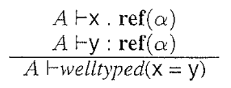
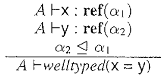
x = y
points-to(x) \( \supseteq \) points-to(y)
points-to(y) \( \supseteq \) points-to(x)
where x can be of the form: x, *x
y can be of the form: y, *y, &y
For the statement x=y, merge the points-to sets of x and y.
Steensgaard's Analysis
p1 = &a
p2 = &b
p1 = p2
r = &p1
p3 = *r
p2 = &d
r
p1
p2
a
b
d
p3
Steensgaard's Analysis
p1 = &a
p2 = &b
p1 = p2
r = &p1
p3 = *r
p2 = &d
r
p1
p2
a,b
d
p3
Steensgaard's Analysis
p1 = &a
p2 = &b
p1 = p2
r = &p1
p3 = *r
p2 = &d
r
p1
p2
a,b,d
p3
Type system
- Not to be confused with data types in programs like int, float, boolean, etc.
- Type: A compile-time data structure used to store the points-to information of a node in the graph
-
Type: (\( \alpha \times \lambda \))
- \( \alpha \): describes data locations to which the variable can point to
- \( \lambda \): describes functions to which the variable can point to
Types - Example
a = &x;
b = &y;
c = b;
a
b
c
x
y
\( \bot \)
\( \bot \)
\( \bot \)
\( \bot \)
\( \bot \)
a
b
c
x
y
Variables
Memory Locations
Types
Types - Example
a = &x;
b = &y;
c = b;
a
b
c
x
y
\( \bot \)
\( \bot \)
\( \bot \)
a
b
c
x
y
Variables
Memory Locations
Types
\( \bot \)
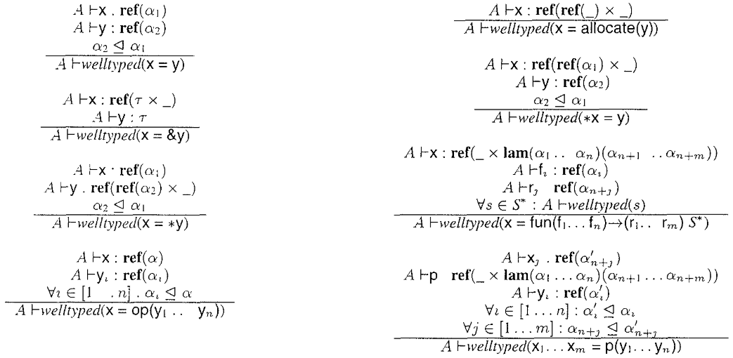
Well Typedness of program
Naive approach
Less constrained approach
a
x
y
\( \bot \)
a
x
y
a
x
y
\( \bot \)
a
x
y
\( \bot \)
\( \bot \)
a = 4
x = a
y = x
m
\( \bot \)
\( \bot \)
\( \bot \)
Well Typedness of program
p1 = &a
p2 = &b
p1 = p2
r = &p1
p3 = *r
p2 = &d
r
p1
p2
a,b,d
p3
r
p1
p2
a
b
d
p3
r
p1
p2
a,b
d
p3
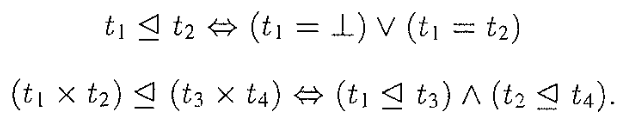
To satisfy \(t1 \trianglelefteq t2\)
- if \(ref(t1) = \bot\) no need to join
- else join \(t1\) and \(t2\)
Well Typedness of program
Steensgaard's Analysis
- Time complexity: O(n)
- Size of each node in the graph - O(1)
- Number of edges from each node - O(1)
- Operation on each node - O(1)
- ~O(1) using union-find data structure
- Number of iterations over the entire graph - O(1)
Andersen vs Steensgaard
r
p1
p2
a
b
d
p3
r
p1
p2
a,b,d
p3
| Time | O(n^3) | O(n) |
|---|---|---|
| Outgoing edges | O(n^2) | O(1) |
| Precision | High | Low |
Results
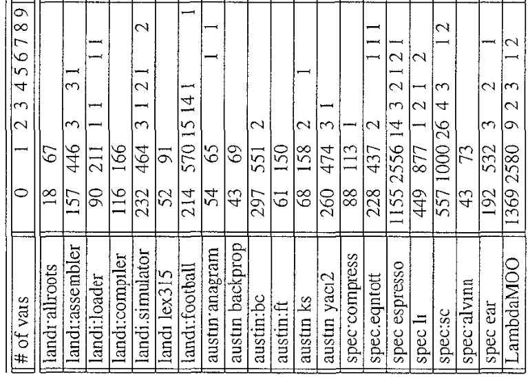
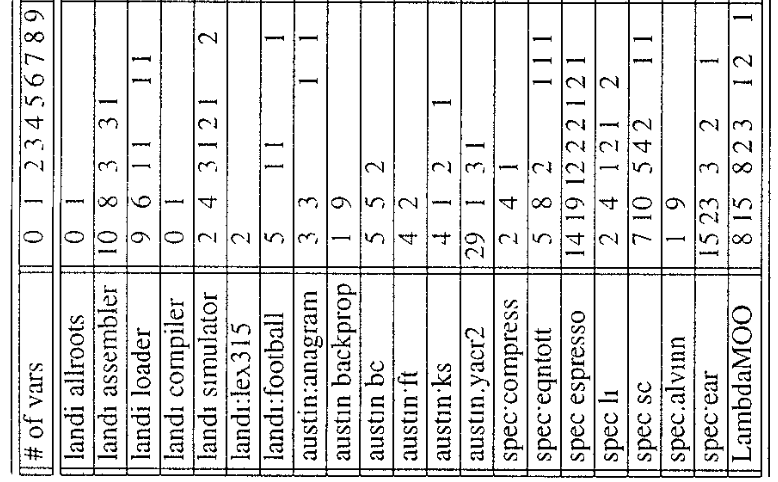
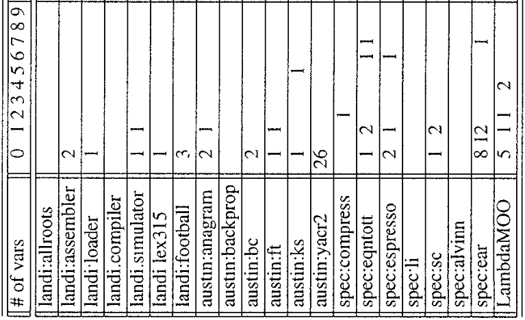
Even with a very conservative analysis, a lot of types point to only one variable.
Summary
- An inter-procedural flow-insensitive points-to analysis
- Computes results in almost linear time
- Uses a type system to describe points-to relations
- Uses a constraint system to describe operations on types
- Imprecise than existing inter-procedural analysis but provides comparable results in less time
Thank You
Every problem in Computer Science can be solved by using another level of indirection.
- David Wheeler