The Arrival
of the
frequent
Outline
Evolution
The arrival of the frequent
Bias in genotype-phenotype maps
Origins of the bias
shaped by
needs
from
causes
genotype-phenotype maps
Evolution
Darwin's idea
(natural selection or survival of the fittest):
things that replicate themselves reliably stick around
Mendel's idea (genes):
in life, genes are the discrete units that replicate (i.e. hold heritable information)
Modern evolutionary synthesis:
Brings the two together into the powerful framework of population genetics.
Wright-Fisher model
The arrival of the frequent: background
Haploid, with mutations and selection
, number of individuals fixed
Individuals at new generation choose parent randomly from previous generation and inherit from it
we add mutations:
when copying the genotype of the parent:
for each one of the L letters,replace it by a random different letter with probability
genotypes are strings of fixed length L over an alphabet with K letters
and selection:
selection coefficient determines the fitness
fitness multiplies the probabilistic weight of an offspring choosing that individual as parent
normalization
The fitness determines the relative number of offspring of different parents
Modern evolutionary synthesis argued for natural selection as the primary force shaping the outcomes of evolution
More recent developments and ideas suggest that developmental bias may also guide evolution.
One way to express developmental bias is via a genotype-phenotype map
One way this bias can affect evolution is via the arrival of the frequent
Genotype-phenotype maps
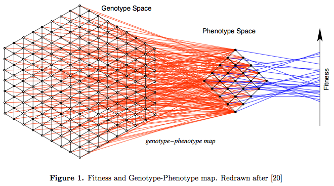
Mutations act on genotypes
Selection acts on phenotypes
The arrival of the frequent: background
From: Schuster, P. A testable genotype phenotype map: Modeling evolution of RNA molecules. In: Lassig, M. and Valleriani, A., editors, Biological Evolution and Statistical Physics, pp. 56{83. Springer-Verlag, Berlin, 2002.
Neutral evolution
Neutral spaces: connected networks of genotypes mapping to same phenotype
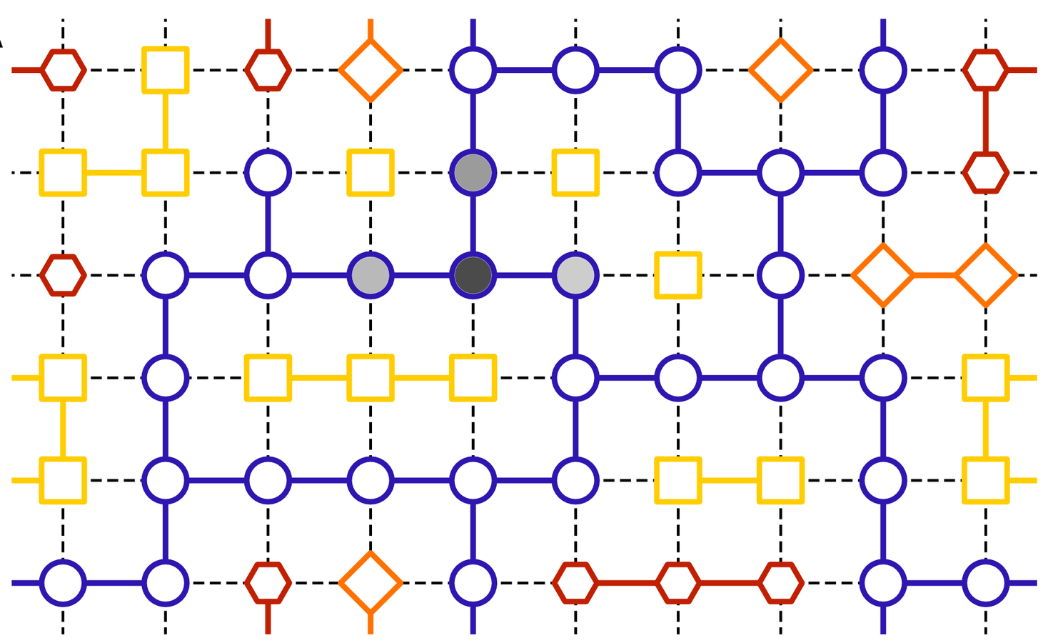
Genotype space, links represent single-point mutations
Neutral exploration: Evolution explores neutral space, being exposed to larger number of neighbouring possibilities, before switching to a different, better, phenotype
The arrival of the frequent: background
Arrival times
The arrival of the frequent
How many generations does it take to find a given phenotype p, starting from phenotype q?
For each set of parents at one generation,
number of p-type offspring at the next generation
follows a Binomial distribution, because each offspring is i.i.d
with mean
, and probability of success
Mean field approximation:
replace by an appropriate average
Probability at least one offpsring of type p:
Arrival times
The arrival of the frequent
Median arrival time:
is calculated differently in different regimes. A particularly easy regime is the polymorphic limit, where the population is spread over the whole neutral space at each generation. Then
where, is the probability that a one-point mutation leads to a phenotype p genotype, averaged over all genotypes in q's neutral space
The arrival of the frequent
Define the phenotype frequency
as the fraction of genotypes that map to phenotype p.
If neutral spaces sufficiently large,
Therefore, approximately,
Frequent phenotypes arrive faster!
and therefore, often before unfrequent phenotypes
See more at: The Arrival of the Frequent: How Bias in Genotype-Phenotype Maps Can Steer Populations to Local Optima
The arrival of the frequent refers to the non-equilibrium phenomenon of arriving, but it can have very significant effects in evolutionary outcomes.
The arrival of the frequent
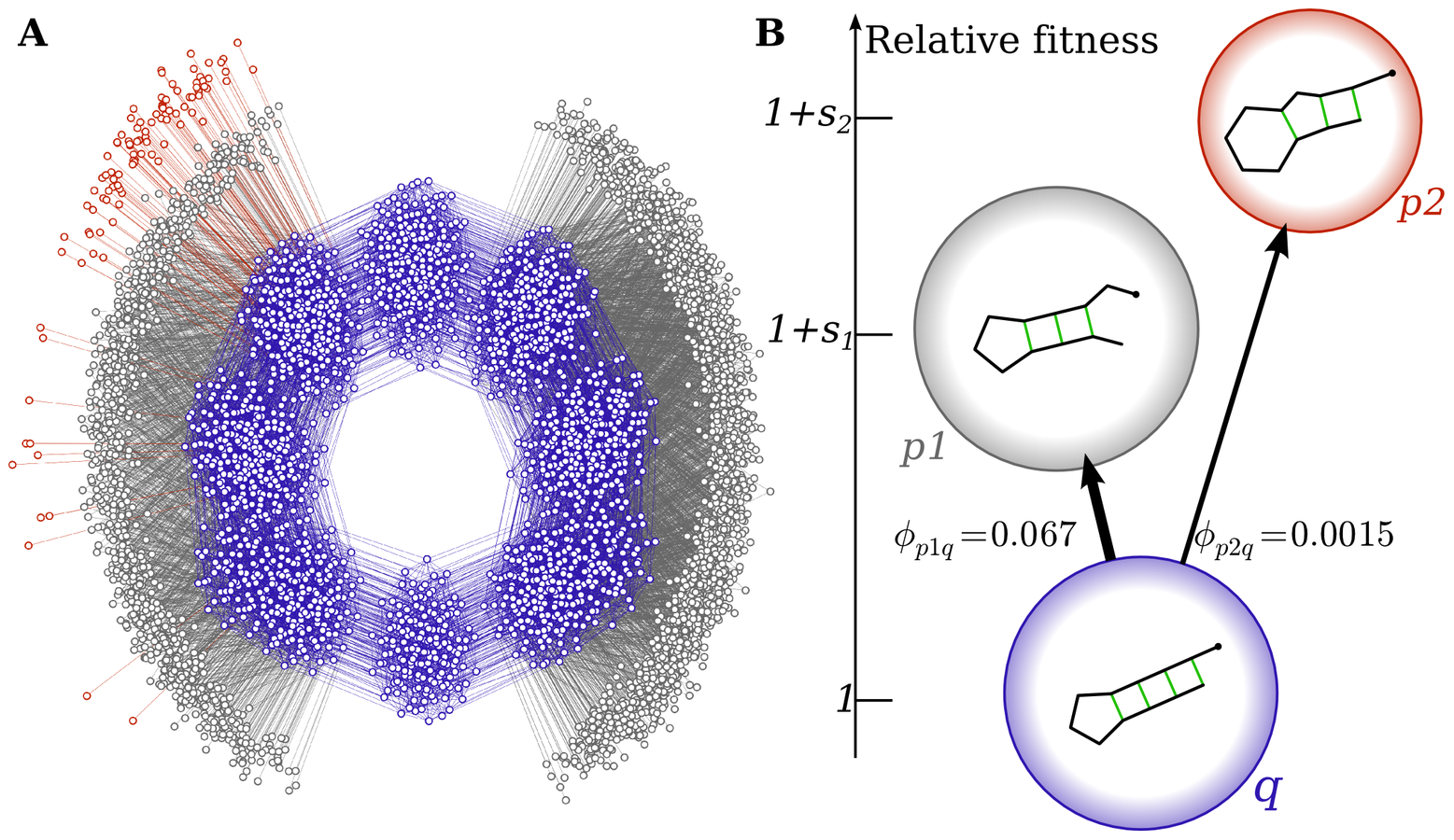
Phenotype 1 is more likely to fix
because it will be "discovered" many more times
Eventually, p2 would arrive and fix, but the environment is likely to have changed by then.
Bias in GP maps
many GP maps have been found to show large biases towards a small number of phenotypes
Nature seems to have fixed on these few most frequent phenotypes
Other alternatives, maybe better ones, may just have never arrived.
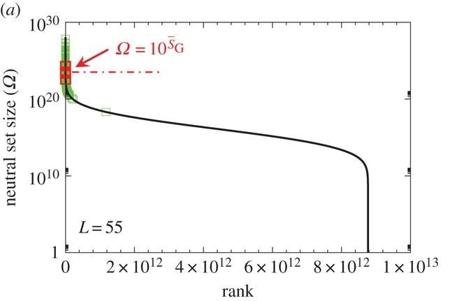
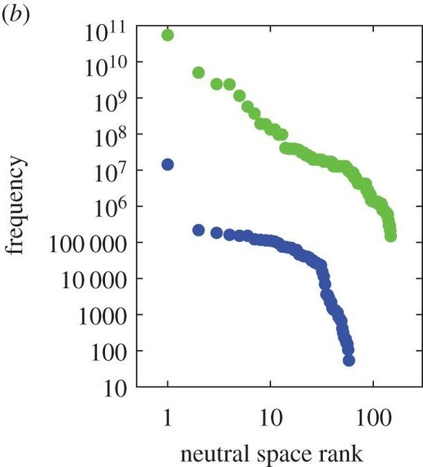
The structure of the genotype–phenotype map strongly constrains the evolution of non-coding RNA
A tractable genotype–phenotype map modelling the self-assembly of protein quaternary structure
Images from:
Bias in GP maps
In the GP maps studied frequent (large neutral set) phenotypes also tend to have:
- higher mutationally robustness
- higher phenotypic evolvability
Surprisingly they also tend to be more simple, as measured by Kolmogorov complexity. This can also make the phenotype more environmentally robust.
All of these things are beneficial for an organism, so GP map bias may explain
why evolution is so effective
Simplicity bias in GP maps
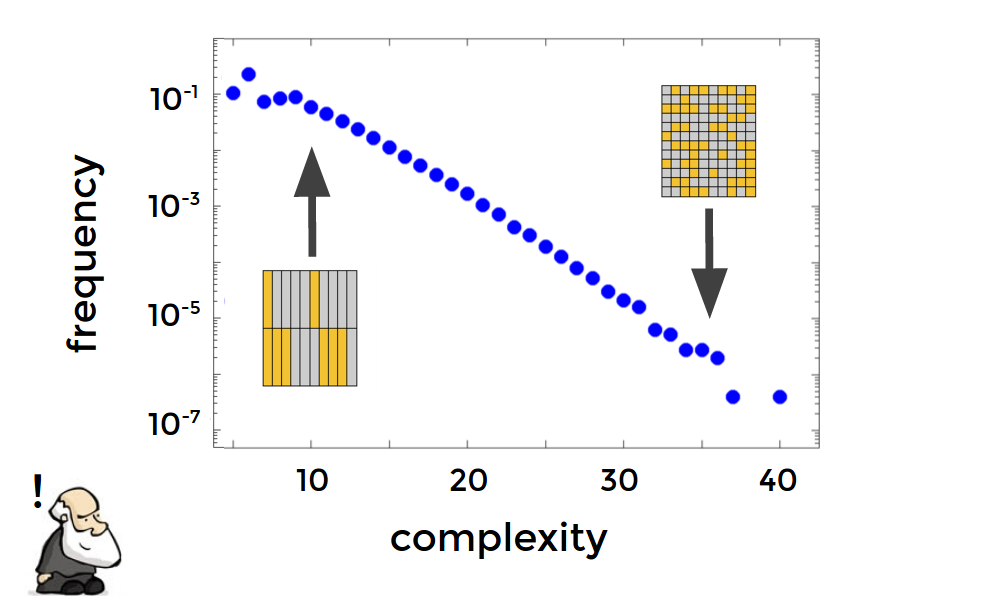
Example: Boolean network model of genetic regulatory networks
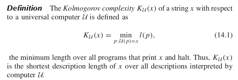
Complexity:
Image by Chico Calmargo
Origin of the bias
Idea 1: Genotype code has constrained and unconstrained parts
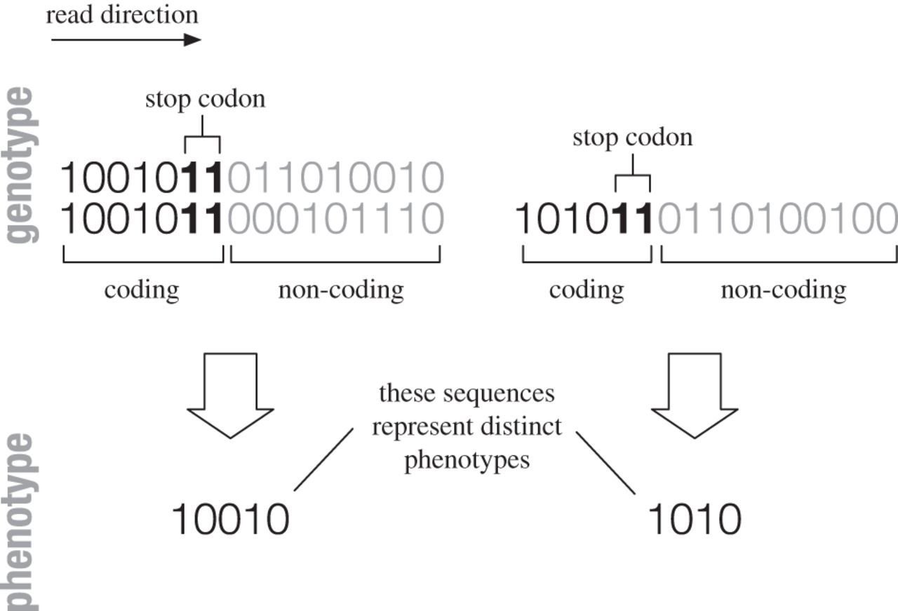
Simplest model:
Fibonacci GP map
Phenotypes with shorter contrained/coding part have larger neutral spaces
and are also more robust, evolvable, and are trivially simpler!
Origin of the bias
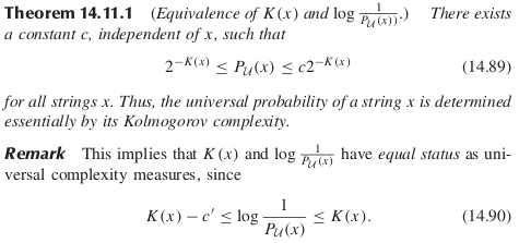
Idea 2: Shannon-Fano-Elias code and the coding theorem
Origin of the bias
Idea 3: Random finite state transducer

A way of describing computable maps,
with a simple parameter describing the complexity of the map: number of states
Origin of the bias
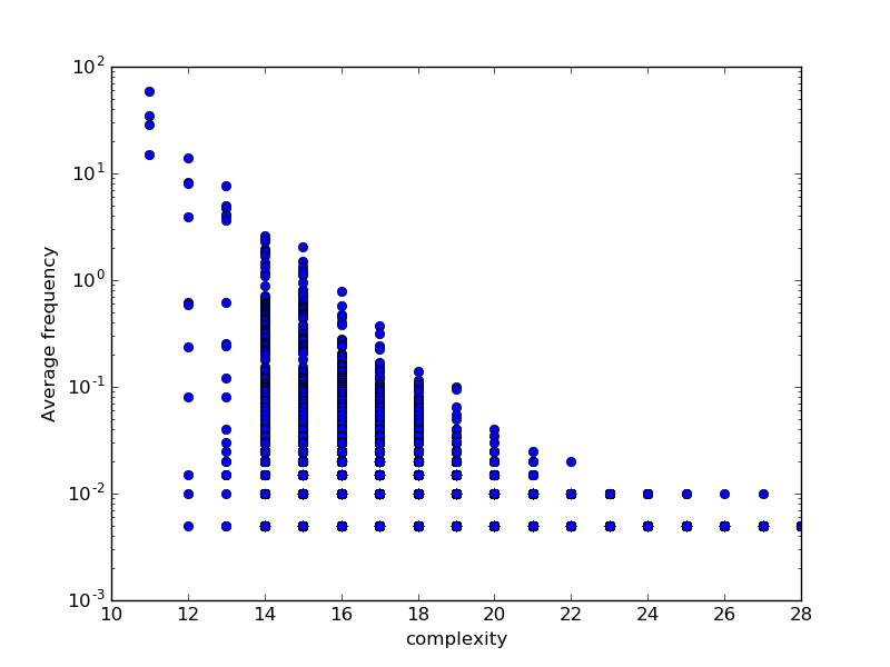
Random finite state transducers show bias!
At least simple ones (4 or 5 states in this case)
Origin of the bias
Bias in finite transducers: why?
How often do we expect or ?
111111111
000000000
Non-coding states -> cycles through non-coding states
How often do we expect or ?
101010101
010101010