DNA sequence motif identification using Gibbs sampling
By Rasa, Maxandre, Guillermo
Outline
Regulatory motifs in DNA sequences
Gibbs sampling
DNA motif model
Known motif length
Unknown motif length
Allowing sequences without the motif
Accounting for phylogenetic relations
Directly inferring K
Regulatory motifs
Regulatory motifs are short (5-30 bp) DNA regions that are located near genes to influence their level of expression.
Since these regions are functionally important, they are considered to be highly conserved between species.
So, to detect them, we can look for highly conserved segments in a set of orthologous genes.
Bayesian inference
What is the "best" parameter given data?
- Posterior mean
- Maximum likelihood
- Maximum information
A way to approximate these is to sample the posterior distribution
Bayes theorem
likelihood
prior
model
DNA motifs model
Motif representation
Background model
DNA motifs model
Starting positions of each motif
Total number of sequences
DNA motif model
Probability of sequence
Probability over all sequences
uniform,
because posterior is a simple multinoulli
We choose the Dirichlet distribution because it is conjugate to the multinomial likelihood
Priors and posteriors
Text
is the count of each base at position k of motif
Gibbs sampling
A Markov Chain Monte Carlo method for sampling posterior distributions in Bayesian inference
Problem
Problem:
has a complicated form
so can't compute
so can't sample posterior
Solution:
Gibbs sampling
The key: these have easy functional forms!
mainly because the domains are simpler
sample M
sample s
The sequence of M and s produced is assured to converge to samples from the full posterior
Known motif length
As a simplification, let's start by assuming the length K of the regulatory motif we're looking for is known.
Challenge:
Maximising the quality of our candidate regulatory motif
One parameter can vary:
a that determines our prior belief on M, of the form:
Challenge:
Maximising the quality of our candidate regulatory motif
How do we define the quality of a candidate regulatory motif?
Two possibilities:
1) it is a lot more likely that it is a regulatory motif than not;
2) it stands out in a sequence, i.e. it has a high information content or, equivalently, a low information entropy.
Challenge:
Maximising the quality of our candidate regulatory motif
...each run of the Gibbs sampler will produce:
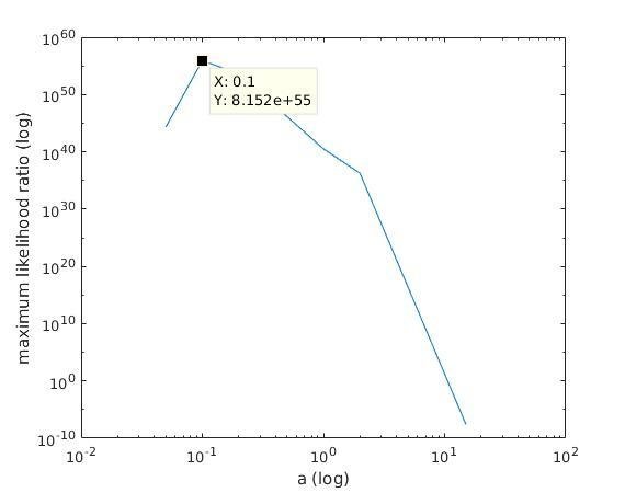
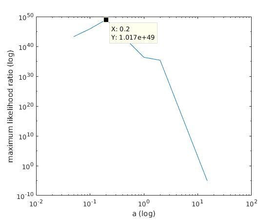
1) a maximum likelihood estimate for M;
2) a minimum entropy estimate for M.
As a result, bear in mind that...
...and a mean of the Ms generated at each iteration of the algorithm (which are sampled from their posterior distribution, as we said previously).
Challenge:
Maximising the quality of our candidate regulatory motif
And so what are we trying to optimise with a?
Two possibilities: find a such that
1) we find the M with maximum likelihood among the different maximum likelihood estimates of M;
2) we find the M with minimum entropy among the minimal entropy estimates of M.
Solution
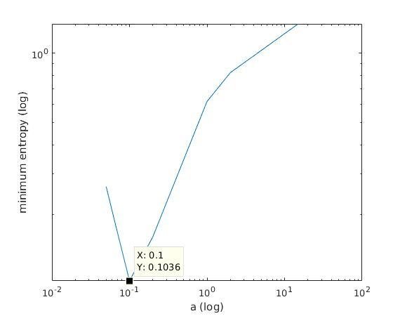
With K = 10:
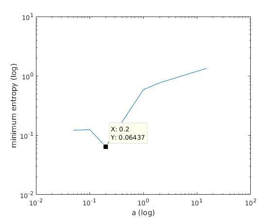
=> M is best
when a ≈ 0.2
With K = 12:
=> M is best
when a ≈ 0.1
Maximum entropy (log)
Maximum likelihood ratio (log)
Maximum entropy (log)
a (log)
a (log)
a (log)
a (log)
Maximum likelihood ratio (log)
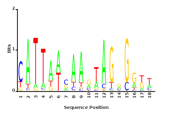
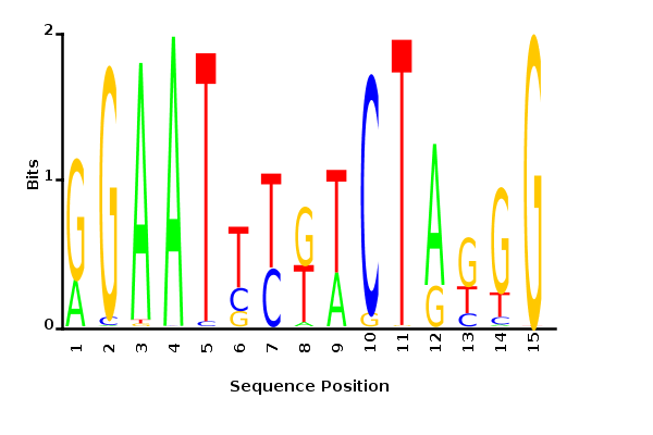
Results
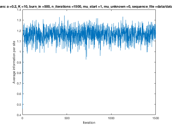
With K = 10 and a = 0.2:
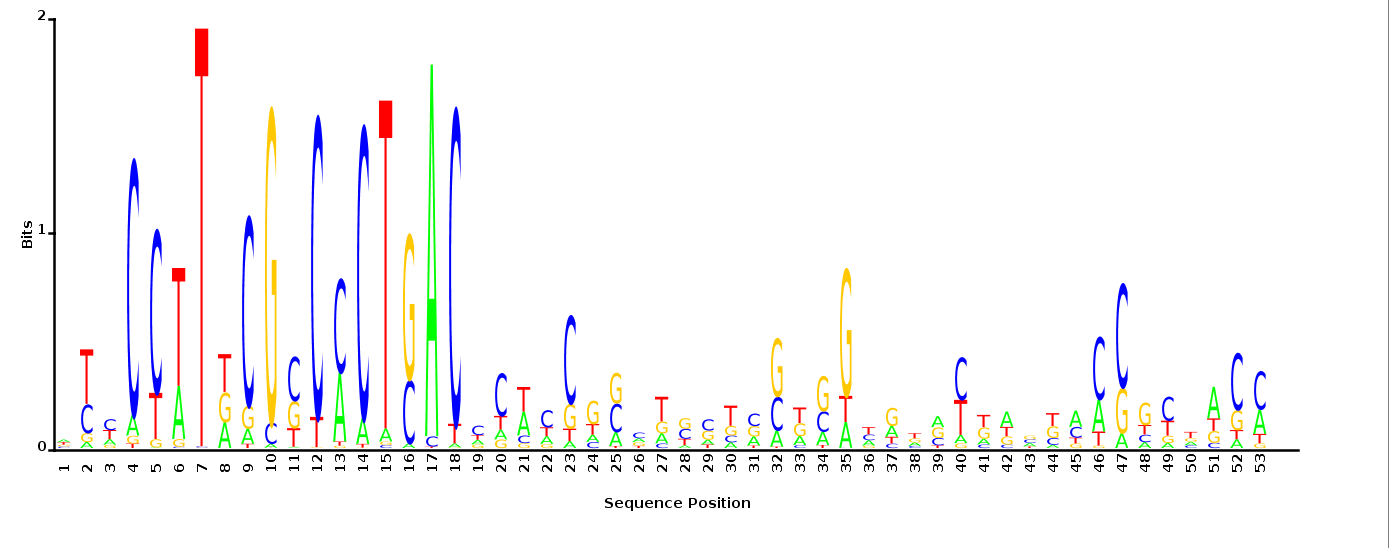
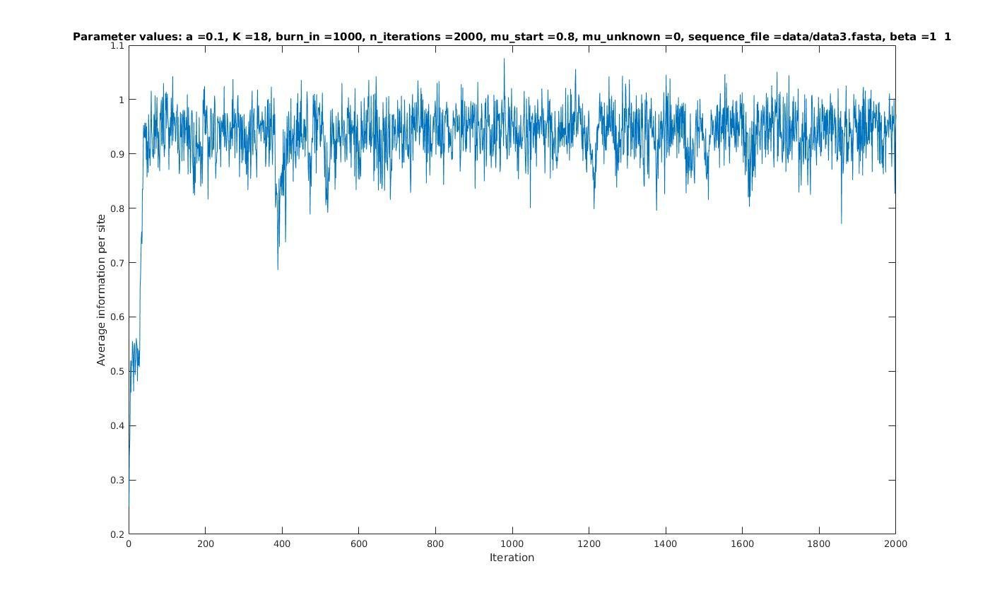
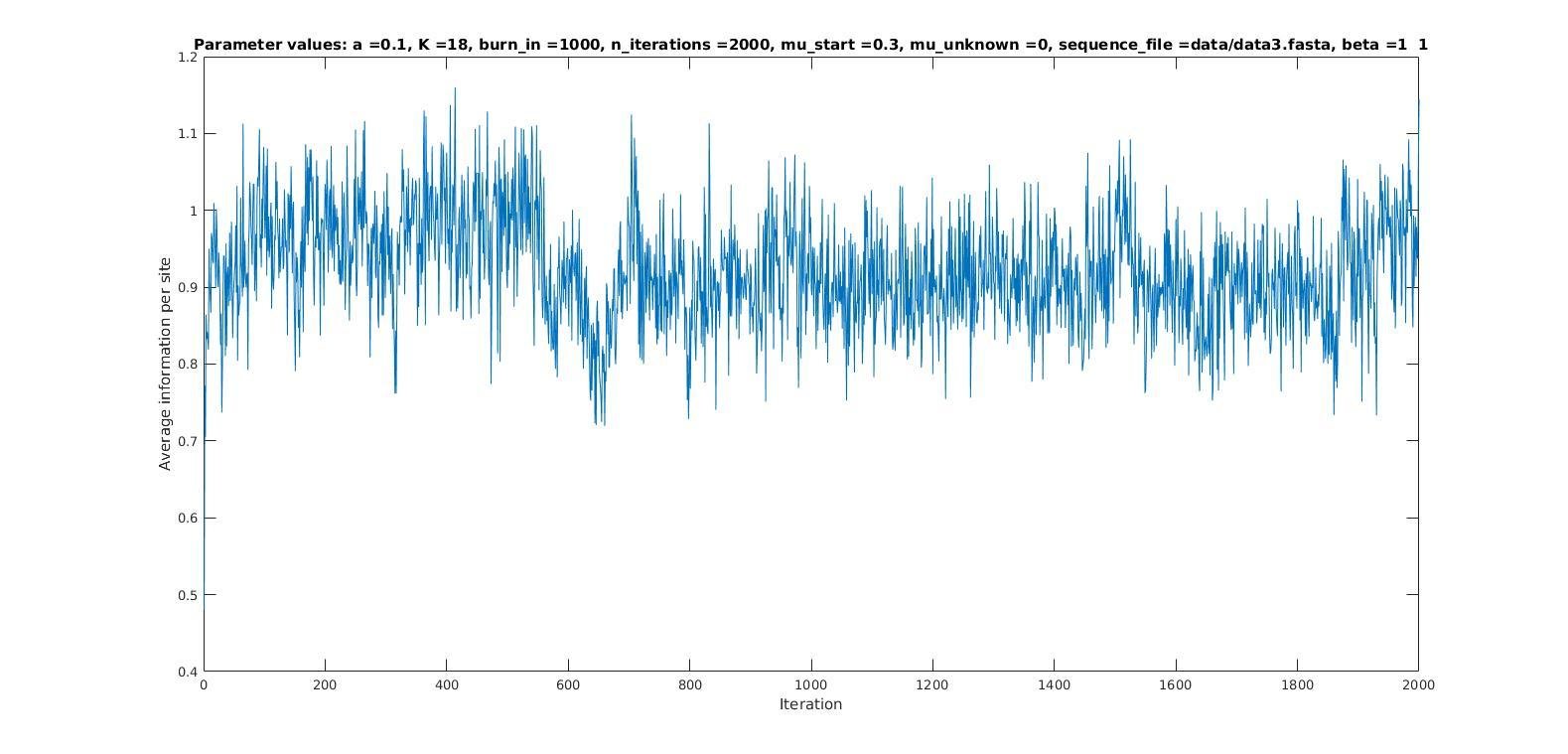
The Gibbs sampler seems to converge very quickly to a motif :
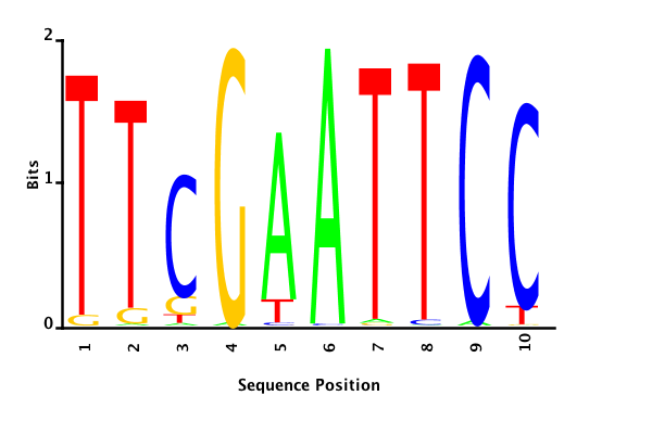
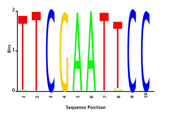
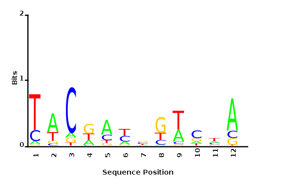
Depending on the criteria we use to select three are possible:
maximum likelihood
minimum entropy
posterior mean
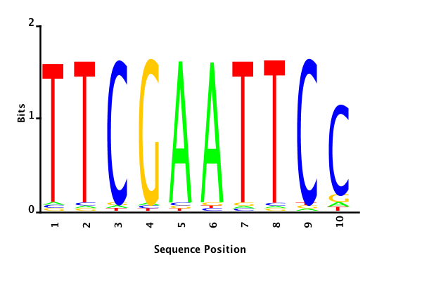
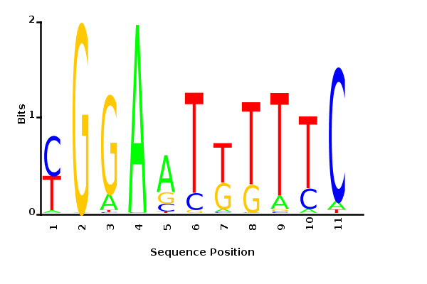
Results
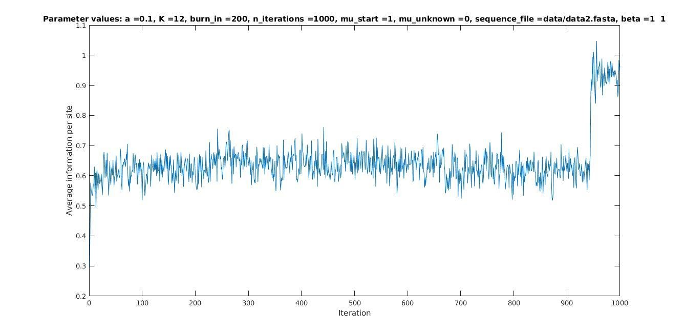
With K = 12 and a = 0.1:
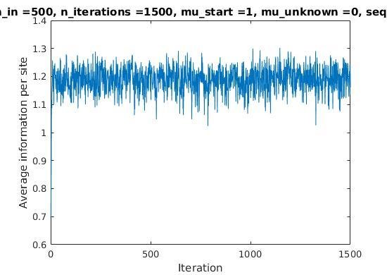
The Gibbs sampler also seems to converge quickly to a motif :
Depending on the criteria we use to select three are possible:
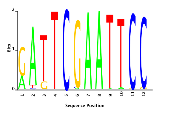
maximum likelihood
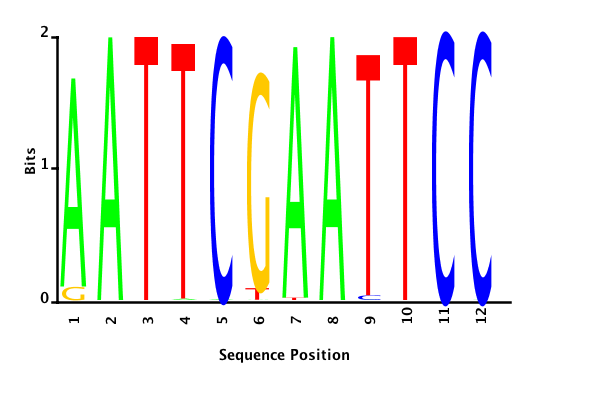
minimum entropy
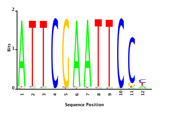
posterior mean
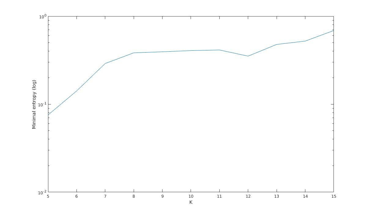
Unknown motif length
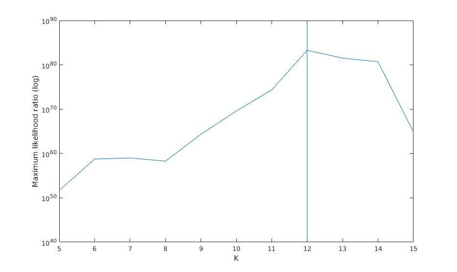
Maximum likelihood ratio versus K
Minimal entropy versus K
Minimal entropy (log)
K
K
Maximum likelihood ratio (log)
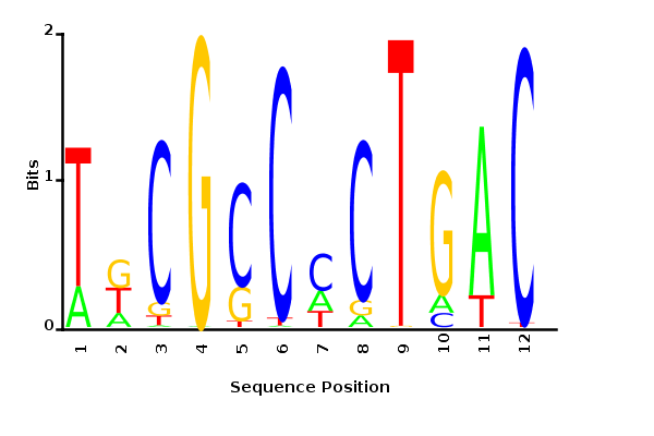
Maximum likelihood PWM
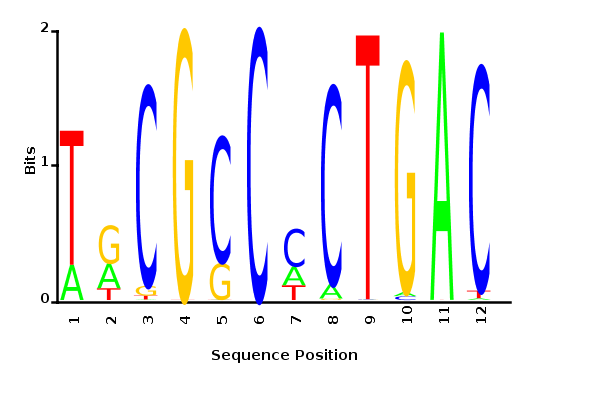
Minimum entropy PWM
Posterior mean PWM
Iterations
Average information
per site
Allowing sequences without the motif
- probability of any sequencing containing a motif
if sequence i contains a motif;
otherwise.
Set
with prob
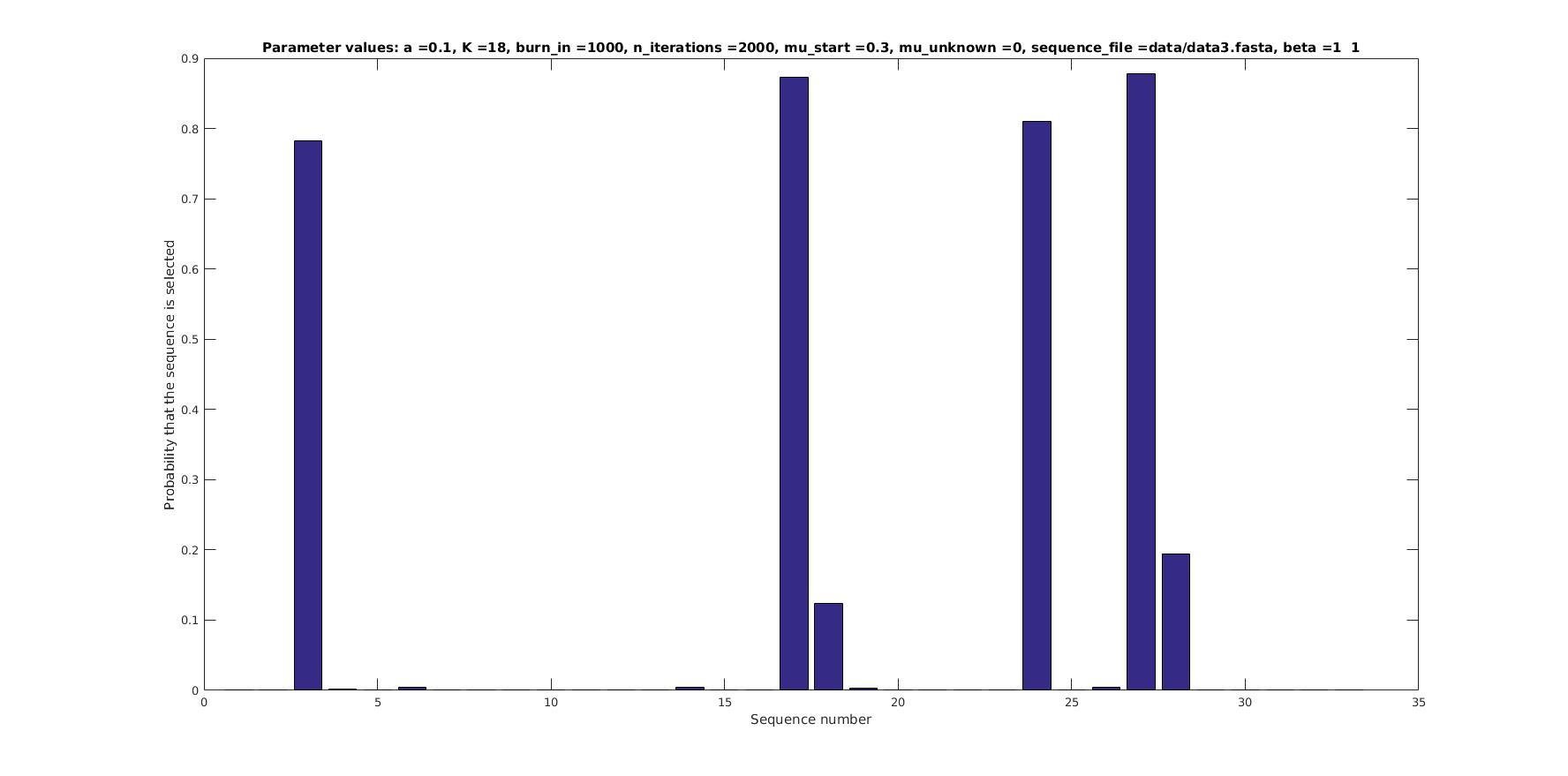
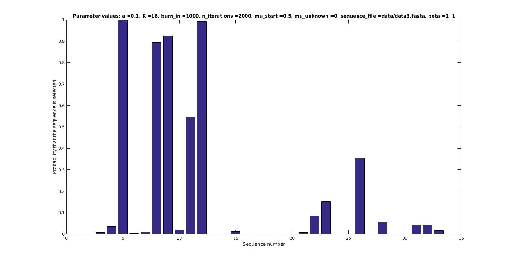
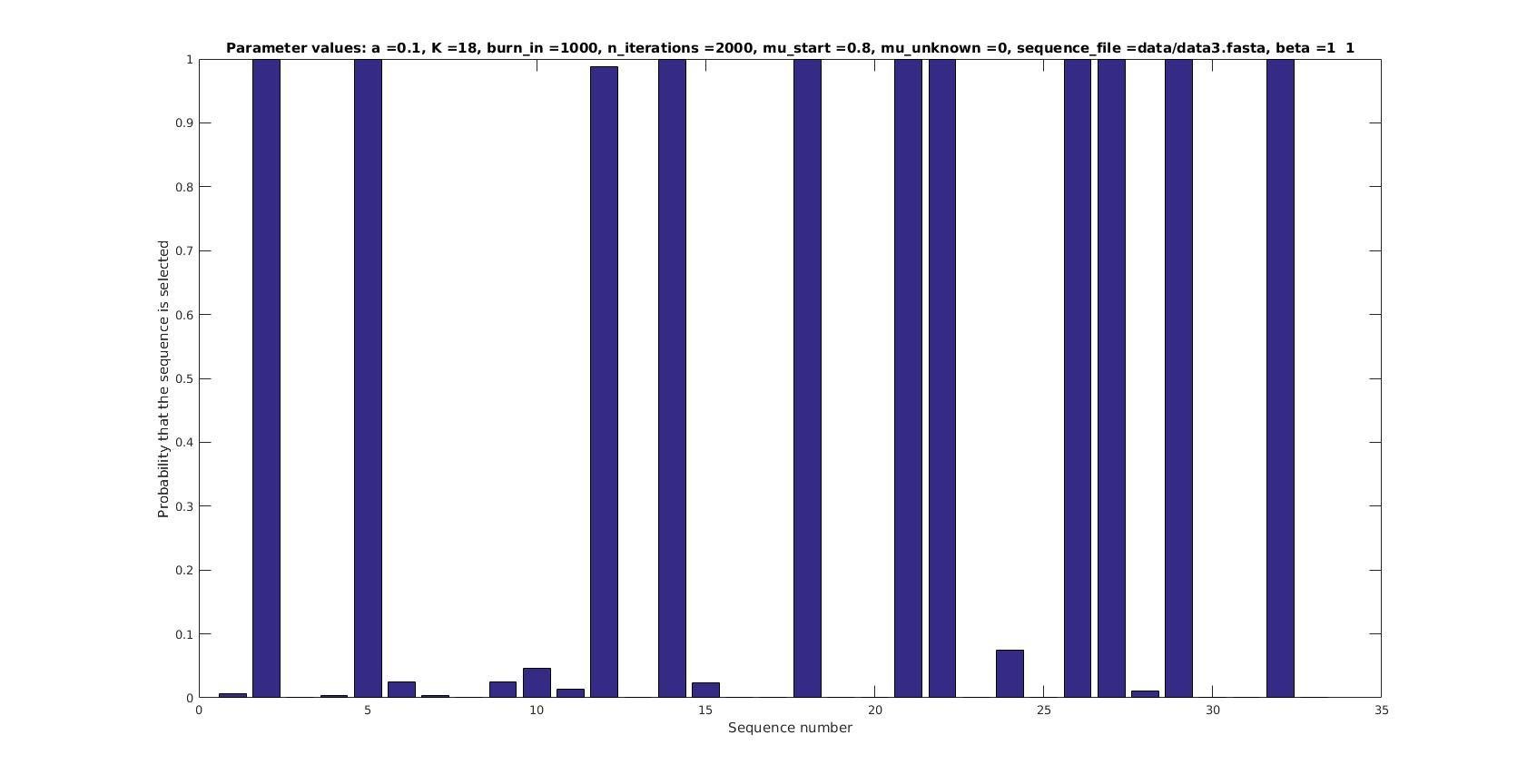
Selected sequences
Actual fraction of
selected sequences:
Sequence number
Sequence number
Sequence number
Probability that sequence is selected
Probability that sequence is selected
Probability that sequence is selected
1
0.9
1
0.9
0.5
0.45
1
0.9
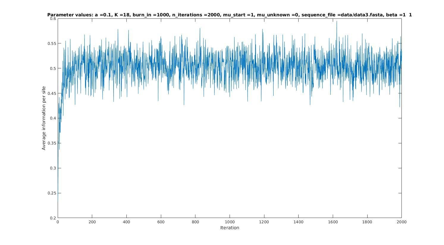
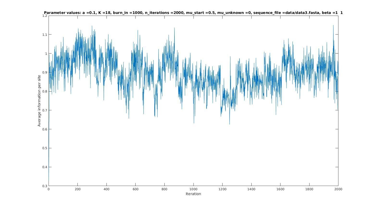
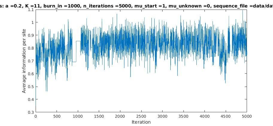
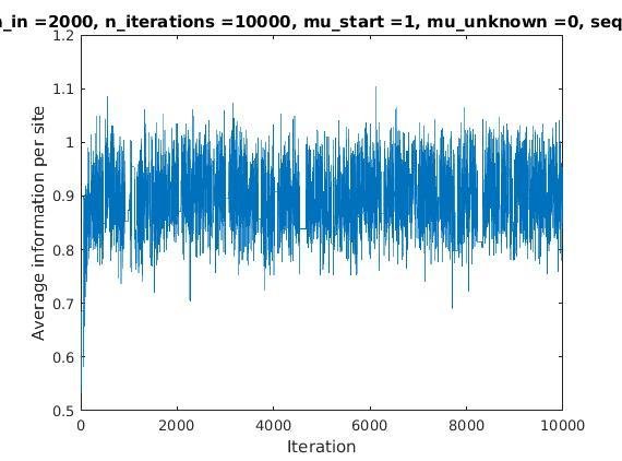
Average information per site versus iteration
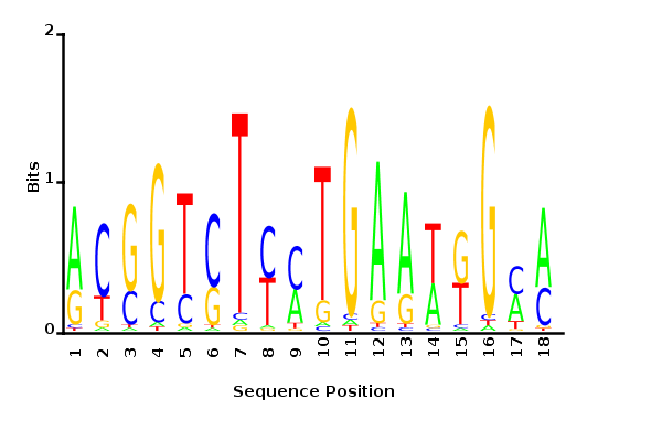
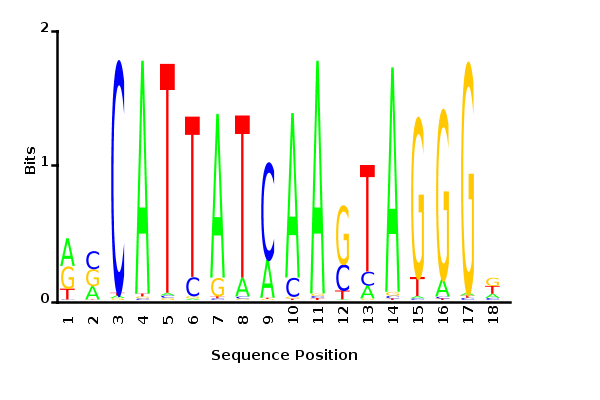
Probability weight matrices
Bayesian inference on the motif probability
Likelihood:
Prior:
Posterior:
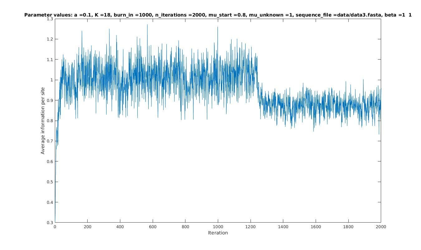
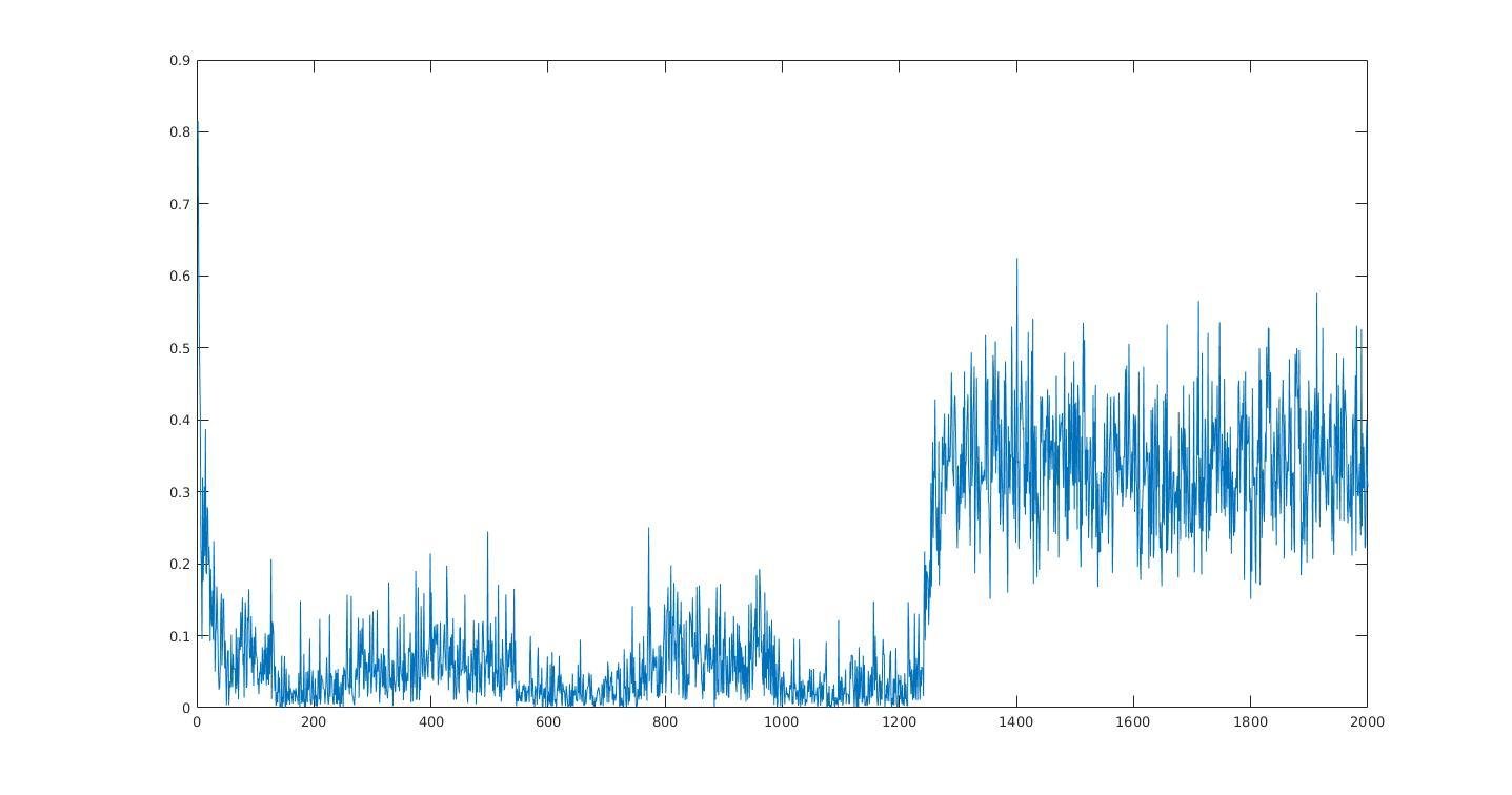
Average information
per site
Iterations
Iterations
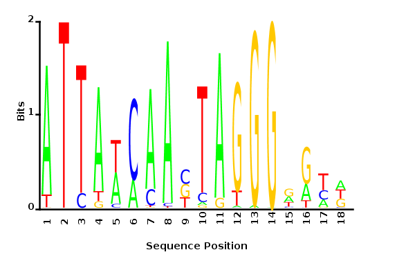
Maximum likelihood-ratio PWM
Analysis of parameter a
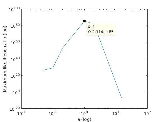
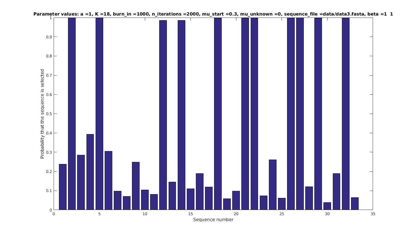
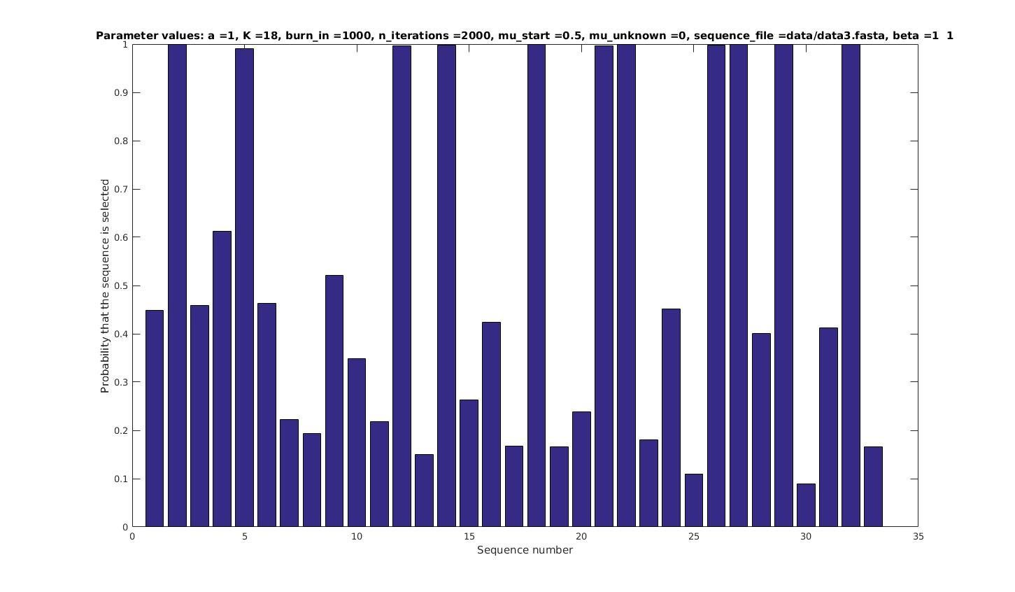
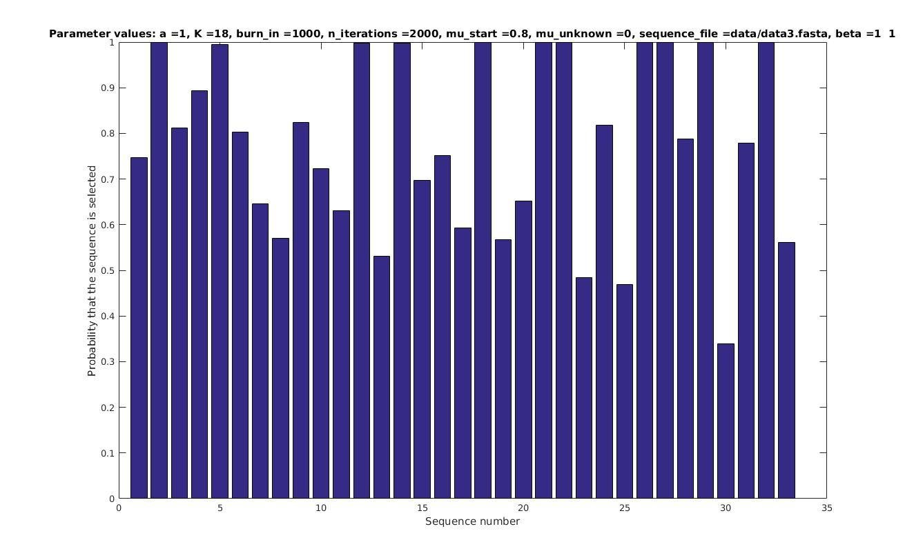
Selected sequences
Sequence number
Sequence number
Sequence number
Probability that sequence is selected
Probability that sequence is selected
Probability that sequence is selected
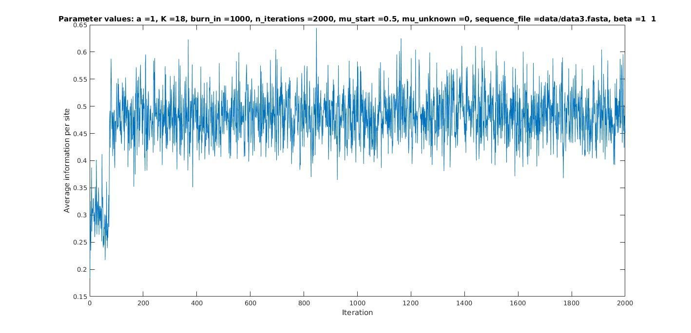
Average information
per site
Iterations
0.5
Accounting for phylogenetic relations
We are given phylogenetic tree
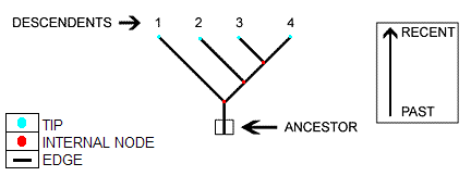
We model evolution for each base pair independently, using the Felsenstein model
We assume the motif represented by M, is the ancestor of all current sequences
Can then use a recursive algorithm for computing the likelihood
Problem
now has a very complicated functional form
Solution: Metropolis-Hastings
Sample using proposal probability
Accept with probability
this should converge to samples from full posterior
Directly inferring K
Try to sample K
Can't find the normalization constant, so use Metropolis-Hastings
Prior for K?
Geometric distribution has maximum entropy for positive integers.
But, K is constrained to be smaller than a certain value, given the sequences, and the starting positions s.
