Evolutionary and Reinforcement Learning Approaches for GW Data Analysis
He Wang
2026/01/27 | Flash Talk
GWFREERIDE: Carving the AI Gradient in Gravitational-Wave Astronomy
International Centre for Theoretical Physics Asia-Pacific (ICTP-AP)
University of Chinese Academy of Sciences (UCAS)


hewang@ucas.ac.cn
Evolutionary and Reinforcement Learning Approaches
for Gravitational-Wave Data Analysis
He Wang
International Centre for Theoretical Physics Asia-Pacific (ICTP-AP)
University of Chinese Academy of Sciences (UCAS)
2026/01/23 · Flash Talk
GWFREERIDE: Carving the AI Gradient in Gravitational-Wave Astronomy
Adaptive trajectory, not a single optimum
Abstract
Upcoming challenges such as MLGWSC2, currently at the proposal stage, provide a new testbed for exploring machine-learning–based approaches to gravitational-wave analysis. In this flash talk, I briefly introduce my core ideas and experience using evolutionary algorithms, Evo-MCTS, and reinforcement learning as adaptive search and optimization tools. I outline key methodological insights and discuss how these ideas may inform future GW analysis tasks, including potential applications to LISA.
才翻到上面看到有人现场拍照 [破涕为笑],随手分享一下
- 我最近常用的PPT英语字体是 Economica,是一个风格比较现代的无衬线字体:https://fonts.google.com/specimen/Economica
- 但用这个字体显得好看,牺牲了一点儿清晰度,有需要的时候还是会回归Helvetica Neue
- 衬线字体我喜欢用 Arno Pro: https://fonts.adobe.com/fonts/arno
- 中文字体已经锁死了喜鹊宋或者木叶(收费字体)
- 颜色一般从MetBrewer里面挑,但并没有特别注意配色:https://github.com/BlakeRMills/MetBrewer
- 今天刚和邵老师说,可能是中年危机的一种表现,就现在越来越喜欢五颜六色的东西。。。也体现在了PPT上。这个完全见仁见智。
- 如果有人对这种PPT感兴趣,我把一个7月份会议的短PPT分享在这供参考:https://www.dropbox.com/scl/fi/duez2bpbcck4ogtn98sw6/songhuang_sesto_20250707.key?rlkey=g18rnjym1hpzke3jxcj5y6ezh&st=ot5xu2w8&dl=0
- 我自己现在习惯的PPT排版的风格只适合分steps展示,不能一次都show全。我自己开始使用这个风格是上课以后,需要满足PPT好看,能吸引注意力,但同时信息量够足,学生可以拿来复习。暂时觉得还好,但过两年可能还是会学着做简单一点儿。
- 用字体大小和颜色来highlight关键词是最简单粗暴、最俗的引导视线的方法,属于广告里早就用烂了的。其实有更好的设计语言,但不会。。。
- PPT风格纯属个人审美兴趣,和报告水平,更和报告内容好坏无关。
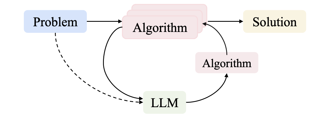
When LLMs Enter the Algorithmic Loop
The LLM does not predict answers — it reshapes how we search for algorithms.
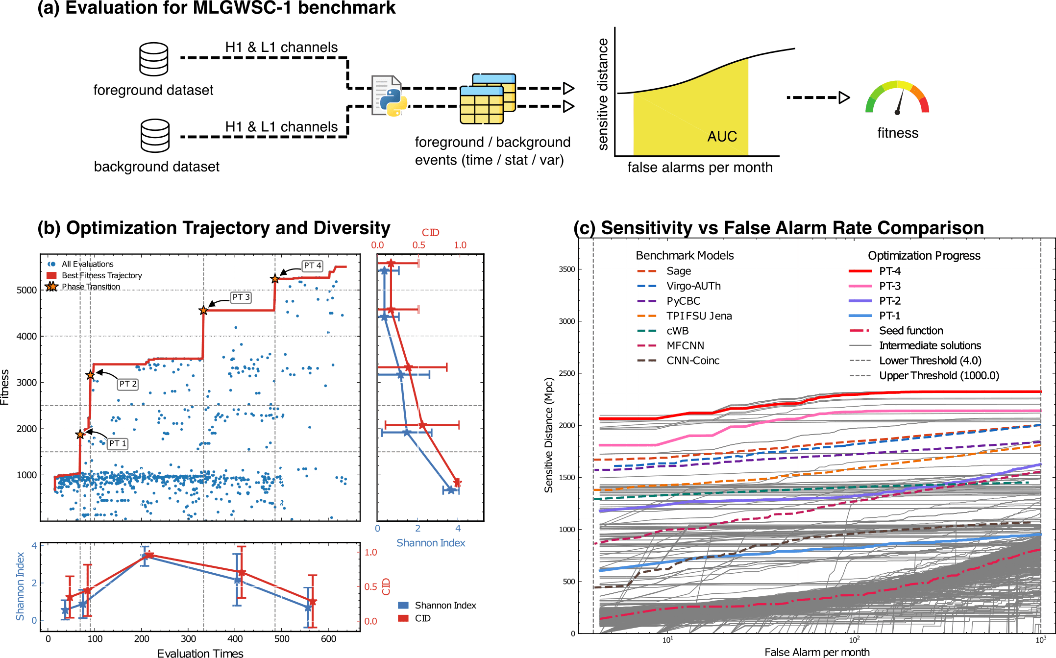
Evaluation for MLGWSC-1 benchmark
LLMs act as policies over algorithms, not predictors of data.
Concept
Mechanism
problem → algorithm
data → algorithm → reward
↺ LLM-guided algorithm updates
from problem-solving to algorithm discovery
HW, LZ. arXiv:2508.03661 [cs.AI]
When LLMs Enter the Algorithmic Loop
The LLM does not predict answers — it reshapes how we search for algorithms.
external_knowledge
(constraint)
PyCBC (linear-core)
cWB (nonlinear-core)
Simple filters (non-linear)
CNN-like (highly non-linear)
Benchmarking against state-of-the-art methods
Evaluation for MLGWSC-1 benchmark
LLM as designer
arXiv:2410.14716 [cs.LG]
HW, LZ. arXiv:2508.03661 [cs.AI]
LLMs act as adaptive policy priors over algorithmic decisions.
Evo-MCTS: When LLMs Enter the Algorithmic Loop
The LLM does not predict answers — it shapes the search process itself.
-
LLM proposes moves, not outputs
-
Search history becomes reusable knowledge
-
Algorithm behavior evolves, not just parameters
What changed?
-
LLMs do not predict waveforms or labels
-
LLMs propose actions that guide the search
-
Evaluations (fitness/likelihood) become reusable memory
Search trajectories matter more than isolated optima.
When LLMs Enter the Algorithmic Loop
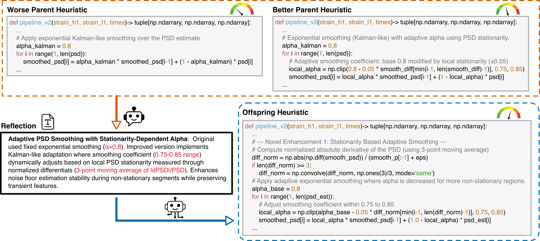
LLM-Driven Algorithmic Evolution Through Reflective Code Synthesis.
HW, LZ. arXiv:2508.03661 [cs.AI]
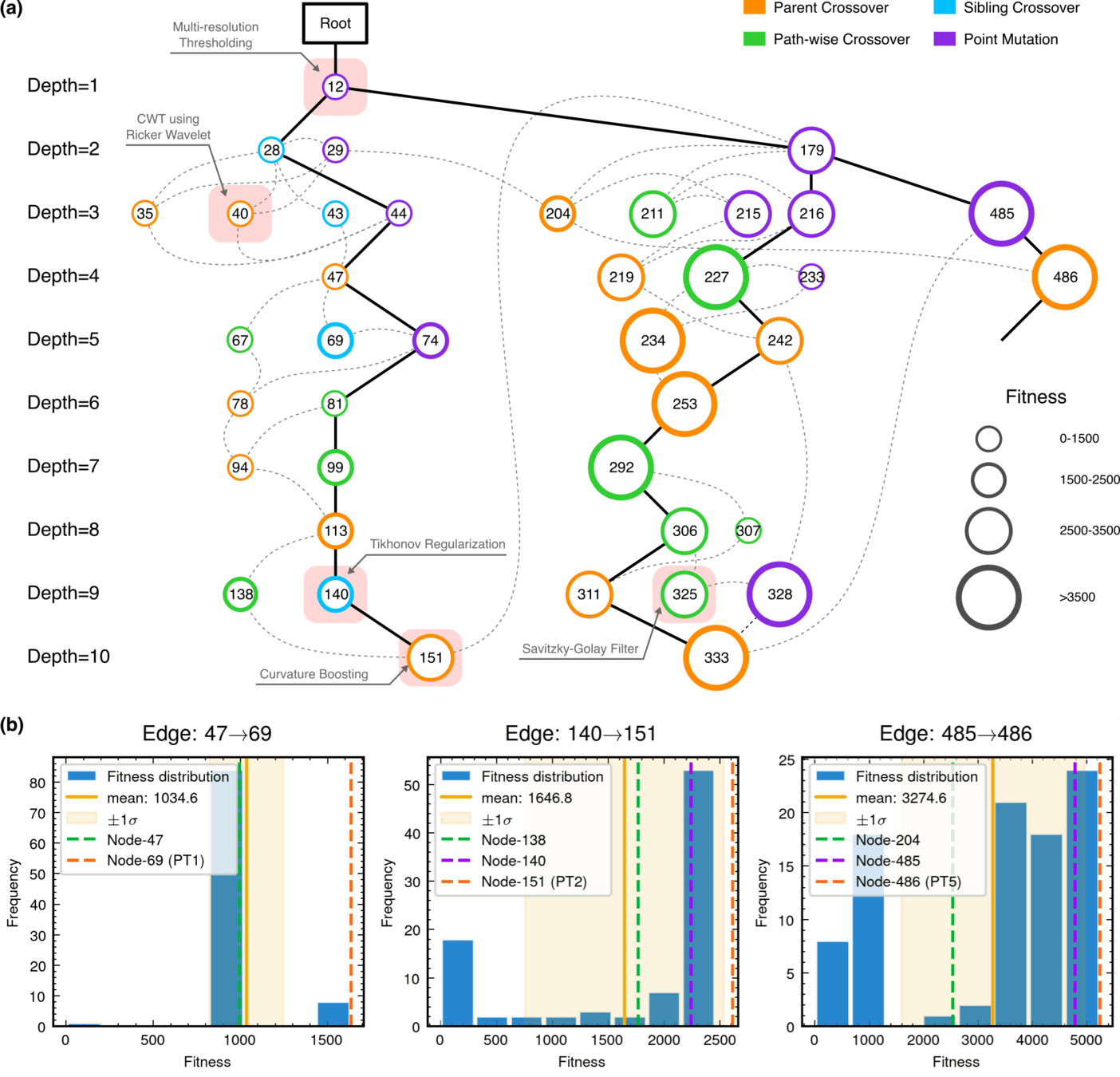
Monte Carlo Tree Search (MCTS) Algorithmic Evolution Pathway
What changed?
-
LLMs propose actions that guide the search
-
Evaluations (fitness/likelihood/...) become reusable memory
Search trajectories matter more than isolated optima.
The LLM does not predict answers — it reshapes how we search for algorithms.
- deepseek-R1 for reflection generation
- o3-mini-medium for code generation
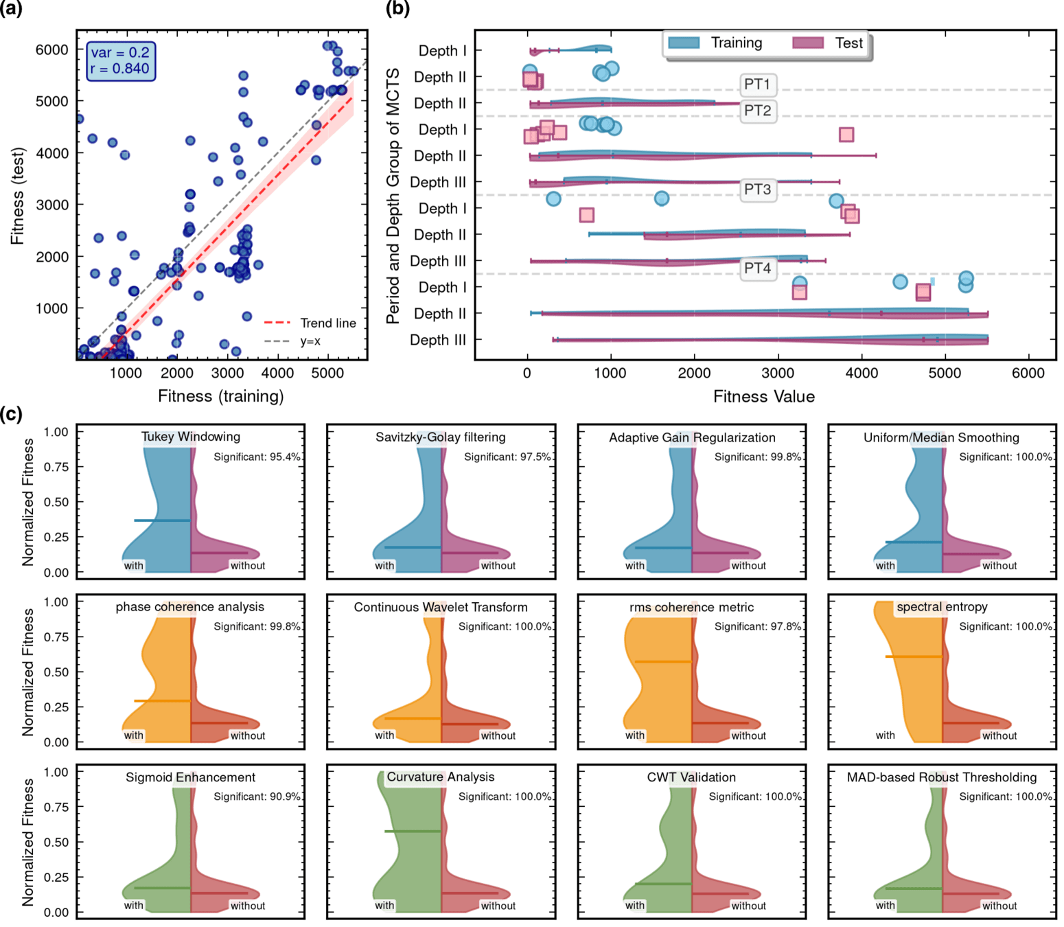
Interpretability Analysis
Algorithmic Component Impact Analysis.
- A comprehensive technique impact analysis using controlled comparative methodology
import numpy as np
import scipy.signal as signal
from scipy.signal.windows import tukey
from scipy.signal import savgol_filter

def pipeline_v2(strain_h1: np.ndarray, strain_l1: np.ndarray, times: np.ndarray) -> tuple[np.ndarray, np.ndarray, np.ndarray]:
    """
    The pipeline function processes gravitational wave data from the H1 and L1 detectors to identify potential gravitational wave signals.
    It takes strain_h1 and strain_l1 numpy arrays containing detector data, and times array with corresponding time points.
    The function returns a tuple of three numpy arrays: peak_times containing GPS times of identified events,
    peak_heights with significance values of each peak, and peak_deltat showing time window uncertainty for each peak.
    """
    eps = np.finfo(float).tiny
    dt = times[1] - times[0]
    fs = 1.0 / dt
    # Base spectrogram parameters
    base_nperseg = 256
    base_noverlap = base_nperseg // 2
    medfilt_kernel = 101       # odd kernel size for robust detrending
    uncertainty_window = 5     # half-window for local timing uncertainty

    # -------------------- Stage 1: Robust Baseline Detrending --------------------
    # Remove long-term trends using a median filter for each channel.
    detrended_h1 = strain_h1 - signal.medfilt(strain_h1, kernel_size=medfilt_kernel)
    detrended_l1 = strain_l1 - signal.medfilt(strain_l1, kernel_size=medfilt_kernel)

    # -------------------- Stage 2: Adaptive Whitening with Enhanced PSD Smoothing --------------------
    def adaptive_whitening(strain: np.ndarray) -> np.ndarray:
        # Center the signal.
        centered = strain - np.mean(strain)
        n_samples = len(centered)
        # Adaptive window length: between 5 and 30 seconds
        win_length_sec = np.clip(n_samples / fs / 20, 5, 30)
        nperseg_adapt = int(win_length_sec * fs)
        nperseg_adapt = max(10, min(nperseg_adapt, n_samples))

        # Create a Tukey window with 75% overlap.
        tukey_alpha = 0.25
        win = tukey(nperseg_adapt, alpha=tukey_alpha)
        noverlap_adapt = int(nperseg_adapt * 0.75)
        if noverlap_adapt >= nperseg_adapt:
            noverlap_adapt = nperseg_adapt - 1

        # Estimate the power spectral density (PSD) using Welch's method.
        freqs, psd = signal.welch(centered, fs=fs, nperseg=nperseg_adapt,
                                  noverlap=noverlap_adapt, window=win, detrend='constant')
        psd = np.maximum(psd, eps)

        # Compute relative differences for PSD stationarity measure.
        diff_arr = np.abs(np.diff(psd)) / (psd[:-1] + eps)
        # Smooth the derivative with a moving average.
        if len(diff_arr) >= 3:
            smooth_diff = np.convolve(diff_arr, np.ones(3)/3, mode='same')
        else:
            smooth_diff = diff_arr

        # Exponential smoothing (Kalman-like) with adaptive alpha using PSD stationarity.
        smoothed_psd = np.copy(psd)
        for i in range(1, len(psd)):
            # Adaptive smoothing coefficient: base 0.8 modified by local stationarity (±0.05)
            local_alpha = np.clip(0.8 - 0.05 * smooth_diff[min(i-1, len(smooth_diff)-1)], 0.75, 0.85)
            smoothed_psd[i] = local_alpha * smoothed_psd[i-1] + (1 - local_alpha) * psd[i]

        # Compute Tikhonov regularization gain based on deviation from median PSD.
        noise_baseline = np.median(smoothed_psd)
        raw_gain = (smoothed_psd / (noise_baseline + eps)) - 1.0

        # Compute a causal-like gradient using the Savitzky-Golay filter.
        win_len = 11 if len(smoothed_psd) >= 11 else ((len(smoothed_psd)//2)*2+1)
        polyorder = 2 if win_len > 2 else 1
        delta_freq = np.mean(np.diff(freqs))
        grad_psd = savgol_filter(smoothed_psd, win_len, polyorder, deriv=1, delta=delta_freq, mode='interp')

        # Nonlinear scaling via sigmoid to enhance gradient differences.
        sigmoid = lambda x: 1.0 / (1.0 + np.exp(-x))
        scaling_factor = 1.0 + 2.0 * sigmoid(np.abs(grad_psd) / (np.median(smoothed_psd) + eps))

        # Compute adaptive gain factors with nonlinear scaling.
        gain = 1.0 - np.exp(-0.5 * scaling_factor * raw_gain)
        gain = np.clip(gain, -8.0, 8.0)

        # FFT-based whitening: interpolate gain and PSD onto FFT frequency bins.
        signal_fft = np.fft.rfft(centered)
        freq_bins = np.fft.rfftfreq(n_samples, d=dt)
        interp_gain = np.interp(freq_bins, freqs, gain, left=gain[0], right=gain[-1])
        interp_psd = np.interp(freq_bins, freqs, smoothed_psd, left=smoothed_psd[0], right=smoothed_psd[-1])
        denom = np.sqrt(interp_psd) * (np.abs(interp_gain) + eps)
        denom = np.maximum(denom, eps)
        white_fft = signal_fft / denom
        whitened = np.fft.irfft(white_fft, n=n_samples)
        return whitened

    # Whiten H1 and L1 channels using the adapted method.
    white_h1 = adaptive_whitening(detrended_h1)
    white_l1 = adaptive_whitening(detrended_l1)

    # -------------------- Stage 3: Coherent Time-Frequency Metric with Frequency-Conditioned Regularization --------------------
    def compute_coherent_metric(w1: np.ndarray, w2: np.ndarray) -> tuple[np.ndarray, np.ndarray]:
        # Compute complex spectrograms preserving phase information.
        f1, t_spec, Sxx1 = signal.spectrogram(w1, fs=fs, nperseg=base_nperseg,
                                              noverlap=base_noverlap, mode='complex', detrend=False)
        f2, t_spec2, Sxx2 = signal.spectrogram(w2, fs=fs, nperseg=base_nperseg,
                                               noverlap=base_noverlap, mode='complex', detrend=False)
        # Ensure common time axis length.
        common_len = min(len(t_spec), len(t_spec2))
        t_spec = t_spec[:common_len]
        Sxx1 = Sxx1[:, :common_len]
        Sxx2 = Sxx2[:, :common_len]

        # Compute phase differences and coherence between detectors.
        phase_diff = np.angle(Sxx1) - np.angle(Sxx2)
        phase_coherence = np.abs(np.cos(phase_diff))

        # Estimate median PSD per frequency bin from the spectrograms.
        psd1 = np.median(np.abs(Sxx1)**2, axis=1)
        psd2 = np.median(np.abs(Sxx2)**2, axis=1)

        # Frequency-conditioned regularization gain (reflection-guided).
        lambda_f = 0.5 * ((np.median(psd1) / (psd1 + eps)) + (np.median(psd2) / (psd2 + eps)))
        lambda_f = np.clip(lambda_f, 1e-4, 1e-2)
        # Regularization denominator integrating detector PSDs and lambda.
        reg_denom = (psd1[:, None] + psd2[:, None] + lambda_f[:, None] + eps)

        # Weighted phase coherence that balances phase alignment with noise levels.
        weighted_comp = phase_coherence / reg_denom

        # Compute axial (frequency) second derivatives as curvature estimates.
        d2_coh = np.gradient(np.gradient(phase_coherence, axis=0), axis=0)
        avg_curvature = np.mean(np.abs(d2_coh), axis=0)

        # Nonlinear activation boost using tanh for regions of high curvature.
        nonlinear_boost = np.tanh(5 * avg_curvature)
        linear_boost = 1.0 + 0.1 * avg_curvature

        # Cross-detector synergy: weight derived from global median consistency.
        novel_weight = np.mean((np.median(psd1) + np.median(psd2)) / (psd1[:, None] + psd2[:, None] + eps), axis=0)

        # Integrated time-frequency metric combining all enhancements.
        tf_metric = np.sum(weighted_comp * linear_boost * (1.0 + nonlinear_boost), axis=0) * novel_weight

        # Adjust the spectrogram time axis to account for window delay.
        metric_times = t_spec + times[0] + (base_nperseg / 2) / fs
        return tf_metric, metric_times

    tf_metric, metric_times = compute_coherent_metric(white_h1, white_l1)

    # -------------------- Stage 4: Multi-Resolution Thresholding with Octave-Spaced Dyadic Wavelet Validation --------------------
    def multi_resolution_thresholding(metric: np.ndarray, times_arr: np.ndarray) -> tuple[np.ndarray, np.ndarray, np.ndarray]:
        # Robust background estimation with median and MAD.
        bg_level = np.median(metric)
        mad_val = np.median(np.abs(metric - bg_level))
        robust_std = 1.4826 * mad_val
        threshold = bg_level + 1.5 * robust_std

        # Identify candidate peaks using prominence and minimum distance criteria.
        peaks, _ = signal.find_peaks(metric, height=threshold, distance=2, prominence=0.8 * robust_std)
        if peaks.size == 0:
            return np.array([]), np.array([]), np.array([])

        # Local uncertainty estimation using a Gaussian-weighted convolution.
        win_range = np.arange(-uncertainty_window, uncertainty_window + 1)
        sigma = uncertainty_window / 2.5
        gauss_kernel = np.exp(-0.5 * (win_range / sigma) ** 2)
        gauss_kernel /= np.sum(gauss_kernel)
        weighted_mean = np.convolve(metric, gauss_kernel, mode='same')
        weighted_sq = np.convolve(metric ** 2, gauss_kernel, mode='same')
        variances = np.maximum(weighted_sq - weighted_mean ** 2, 0.0)
        uncertainties = np.sqrt(variances)
        uncertainties = np.maximum(uncertainties, 0.01)

        valid_times = []
        valid_heights = []
        valid_uncerts = []
        n_metric = len(metric)

        # Compute a simple second derivative for local curvature checking.
        if n_metric > 2:
            second_deriv = np.diff(metric, n=2)
            second_deriv = np.pad(second_deriv, (1, 1), mode='edge')
        else:
            second_deriv = np.zeros_like(metric)

        # Use octave-spaced scales (dyadic wavelet validation) to validate peak significance.
        widths = np.arange(1, 9)  # approximate scales 1 to 8
        for peak in peaks:
            # Skip peaks lacking sufficient negative curvature.
            if second_deriv[peak] > -0.1 * robust_std:
                continue
            local_start = max(0, peak - uncertainty_window)
            local_end = min(n_metric, peak + uncertainty_window + 1)
            local_segment = metric[local_start:local_end]
            if len(local_segment) < 3:
                continue
            try:
                cwt_coeff = signal.cwt(local_segment, signal.ricker, widths)
            except Exception:
                continue
            max_coeff = np.max(np.abs(cwt_coeff))
            # Threshold for validating the candidate using local MAD.
            cwt_thresh = mad_val * np.sqrt(2 * np.log(len(local_segment) + eps))
            if max_coeff >= cwt_thresh:
                valid_times.append(times_arr[peak])
                valid_heights.append(metric[peak])
                valid_uncerts.append(uncertainties[peak])

        if len(valid_times) == 0:
            return np.array([]), np.array([]), np.array([])
        return np.array(valid_times), np.array(valid_heights), np.array(valid_uncerts)

    peak_times, peak_heights, peak_deltat = multi_resolution_thresholding(tf_metric, metric_times)
return peak_times, peak_heights, peak_deltat- Automatically discover and interpret the value of nonlinear algorithms
- Facilitating new knowledge production along with experience guidance
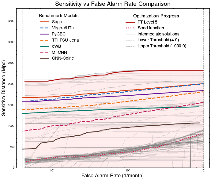
PT Level 5
Framework Mechanism Analysis
Integrated Architecture Validation
- A comprehensive comparison of our integrated
Evo-MCTS framework against its constituent components operating in isolation.- Evo-MCTS: MCTS + Self-evolve + Reflection mech.
- MCTS-AHD: MCTS framework for CO.
- ReEvo: evolutionary framework for CO.
Contributions of knowledge synthesis
- Compare to w/o external knowledge
- non-linear vs linear only
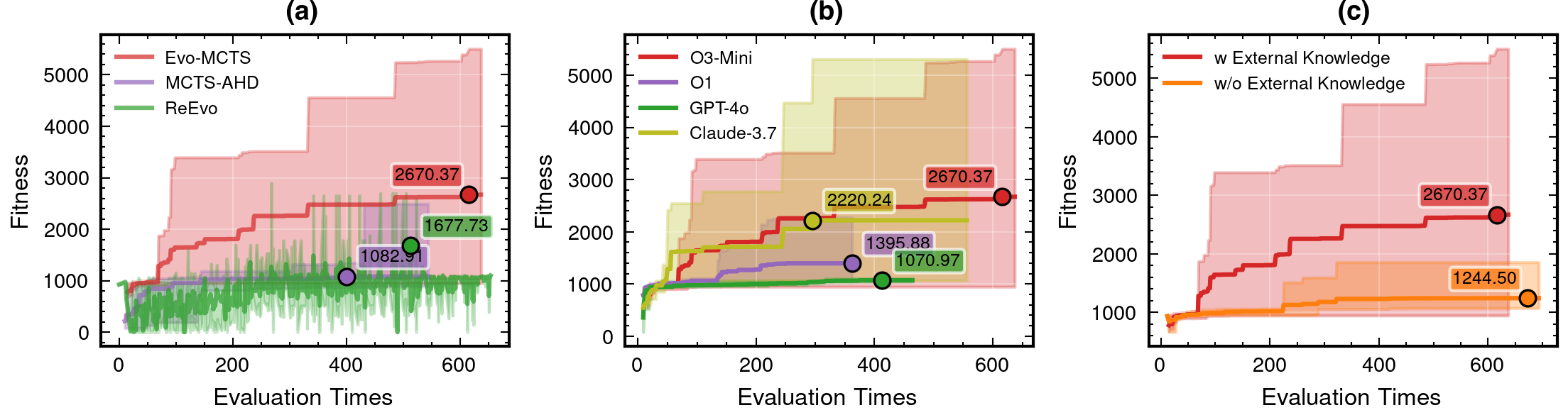
LLM Model Selection and Robustness Analysis
- Ablation study of various LLM contributions (code generator) and their robustness.
-
o3-mini-medium
o1-2024-12-17
gpt-4o-2024-11-20
claude-3-7-sonnet-20250219-thinking
-
59.1%
115%
Framework Mechanism Analysis
AI and Cosmology: From Computational Tools to Scientific Discovery
Contributions of knowledge synthesis
- Compare to w/o external knowledge
- non-linear vs linear only
59.1%
115%
59.1%
### External Knowledge Integration
1. **Non-linear** Processing Core Concepts:
- Signal Transformation:
* Non-linear vs linear decomposition
* Adaptive threshold mechanisms
* Multi-scale analysis
- Feature Extraction:
* Phase space reconstruction
* Topological data analysis
* Wavelet-based detection
- Statistical Analysis:
* Robust estimators
* Non-Gaussian processes
* Higher-order statistics
2. Implementation Principles:
- Prioritize adaptive over fixed parameters
- Consider local vs global characteristics
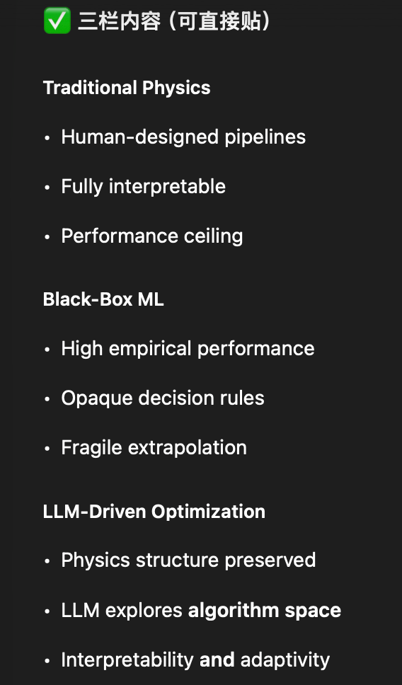
- Balance computational cost with accuracyTraditional Physics
✓ Fully interpretable
✗ Performance ceiling
Human-designed pipelines
Fixed heuristics
Examples:
Matched filtering
χ² tests
Black-box AI
✓ High performance
✗ Opaque decisions
End-to-end prediction
Model-centric learning
Examples:
CNNs, DINGO
Interpretable
Algorithmic Discovery
Algorithms as search objects
Physics-informed objectives
Competitive with state-of-the-art
(MLGWSC-1 benchmark)
Example:
Evo-MCTS (this work)
AlphaEvolve
Interpretable AI for Gravitational-Wave Discovery
Scientific discovery requires interpretability — not just performance.
AI should help us understand why an algorithm works — not just output an answer.

PyCBC (linear-core)
cWB (nonlinear-core)
Simple filters (non-linear)
CNN-like (highly non-linear)
Benchmarking against state-of-the-art methods
(MLGWSC1)
HW, LZ. arXiv:2508.03661 [cs.AI]
Interpretable AI Approach
The best of both worlds
Input
Physics-Informed
Algorithm
(High interpretability)
Output
Example: Evo-MCTS, AlphaEvolve
AI Model
Physics
Knowledge
Traditional Physics Approach
Input
Human-Designed Algorithm
(Based on human insight)
Output
Example: Matched Filtering, linear regression
Black-Box AI Approach
Input
AI Model
(Low interpretability)
Output
Examples: CNN, AlphaGo, DINGO
Data/
Experience
Data/
Experience
🎯 OUR WORK
Scientific discovery requires interpretability, not just performance.
Interpretable AI for Gravitational-Wave Discovery
Scientific discovery requires interpretability — not just performance.
AI should help us understand why an algorithm works — not just output an answer.
Key Takeaways: ... against Symbolic Regression
Any algorithm design problem can be seen as an optimization problem
- Many intermediate processes in gravitational wave data processing can be viewed as "algorithm optimization" problems, such as filter design, noise modeling, detection statistic construction, etc.
- Many analytical modeling and "symbolic regression" methods in theoretical physics and cosmology can also be seen as "algorithm optimization" problems
- Symbolic regression vs algorithm optimization:
- Other Opt. Problem Egs:
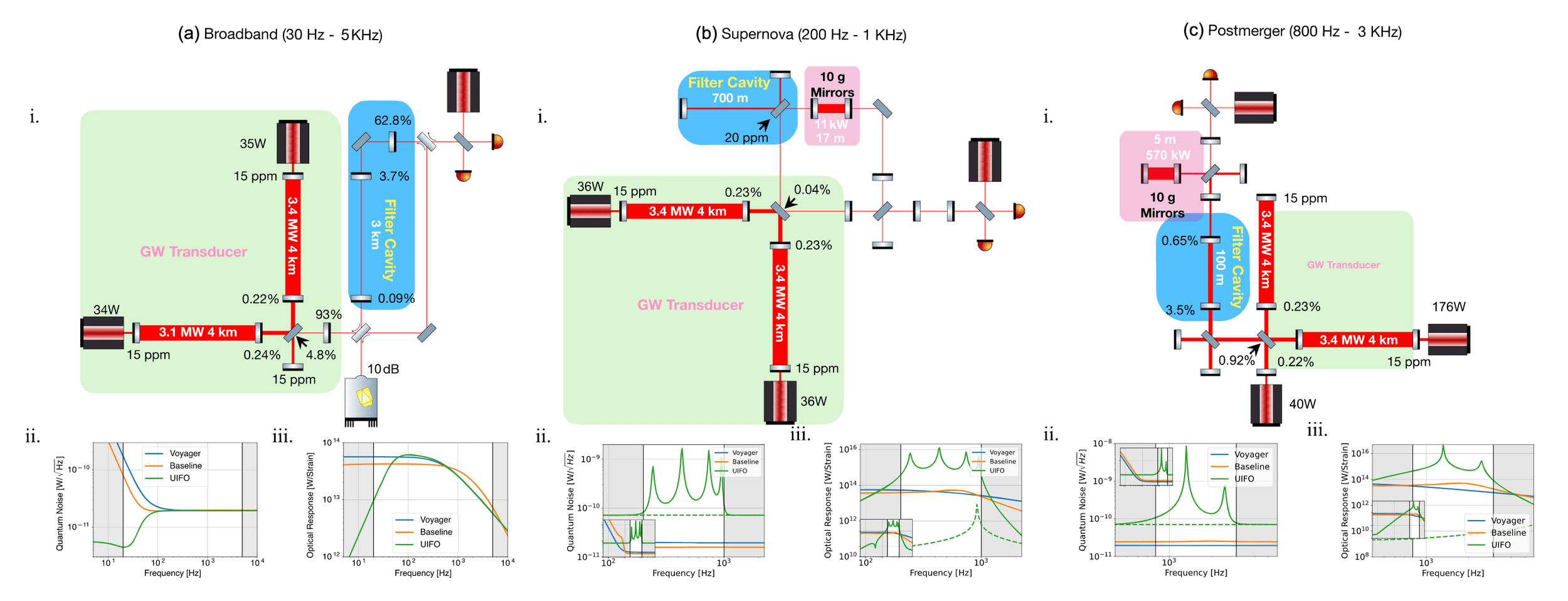
- AI-driven design of experiments. [Phys. Rev. X 15, 021012 (2025)]
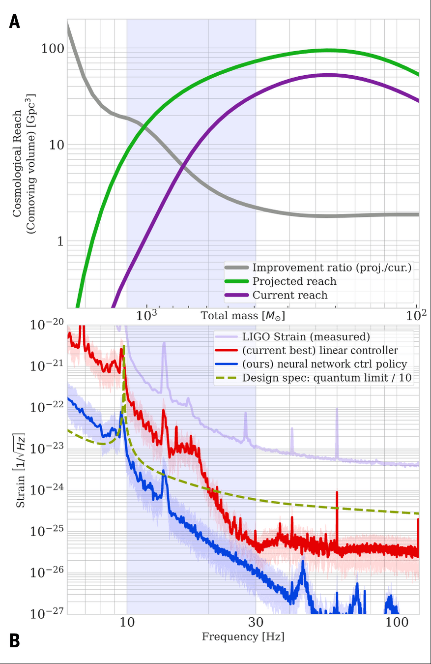
- RL design for multiple filters in LIGO control system. [Science (2025)]

vs
From Black-Box AI to Algorithmic Co-Design
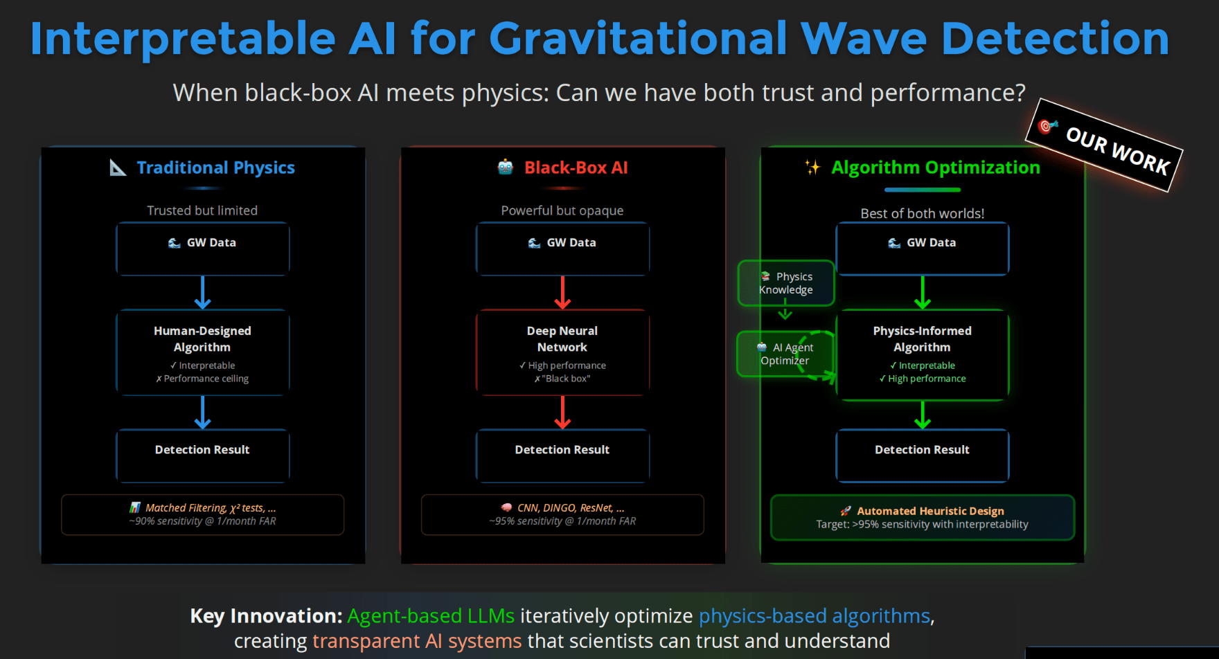
LLMs as agents that optimize physics-based algorithms
A new axis: adaptivity over algorithm design
LLMs allow us to search over algorithms, not just over parameters.
Interpretable AI for Gravitational-Wave Discovery
Scientific discovery requires interpretability — not just performance.
Traditional Physics
✓ Fully interpretable
✗ Performance ceiling
Human-designed pipelines
Fixed heuristics
Examples:
Matched filtering
χ² tests
Black-box AI
✓ High performance
✗ Opaque decisions
End-to-end prediction
Model-centric learning
Examples:
CNNs, DINGO
Interpretable Algorithmic Discovery
✓ Interpretable
✓ High performance
Algorithms as search objects
Physics-informed objectives
Example:
Evo-MCTS (this work)
AI should help us understand why an algorithm works — not just output an answer.
Interpretable AI Approach
The best of both worlds
Input
Physics-Informed
Algorithm
(High interpretability)
Output
Example: Evo-MCTS, AlphaEvolve
AI Model
Physics
Knowledge
Traditional Physics Approach
Input
Human-Designed Algorithm
(Based on human insight)
Output
Example: Matched Filtering, linear regression
Black-Box AI Approach
Input
AI Model
(Low interpretability)
Output
Examples: CNN, AlphaGo, DINGO
Data/
Experience
Data/
Experience
🎯 OUR WORK
What do we think about AI for scientific discovery?
Scientific discovery requires interpretability, not just performance.
Why MLGWSC2 Needs More Than Better Classifiers
From single-pipeline performance to ensemble unbiasedness
We emphasize evaluating complementarity and ensemble behavior rather than single-pipeline superiority.
What LVK already does
-
GWTC catalogs rely on multiple independent pipelines
-
A candidate proceeds if any pipeline produces a confidence trigger
-
-
This already forms an implicit ensemble
Ensembling is already standard practice — just not explicitly analyzed.
The missing question
-
Each pipeline carries distinct inductive biases
(eg: duration, morphology, noise response, parameter coverage).
cWB
GstLAL
PyCBC
AI_1
AI_2
AI_3
AI_n
Is the ensemble unbiased?
LVK anchor pipelines
(selected)
Ensemble evaluation
MLGWSC-2 is under proposal development with active community input (e.g. Nitz, Dent, Messenger, ...).
Related works
- Combining gravitational wave search pipelines with conformal prediction [2402.19313; G2600593]
A RL Perspective on LISA Global Fitting
“I don’t claim this is solved. I claim the framing matters.”
Global fitting is not a single inference — it is a long-horizon control problem.
- Numerical orbits (of Taiji)
- Unequal-arm
- TDI-2.0

preliminary
preliminary
MH Du+, arXiv:2505.16500 [gr-qc]
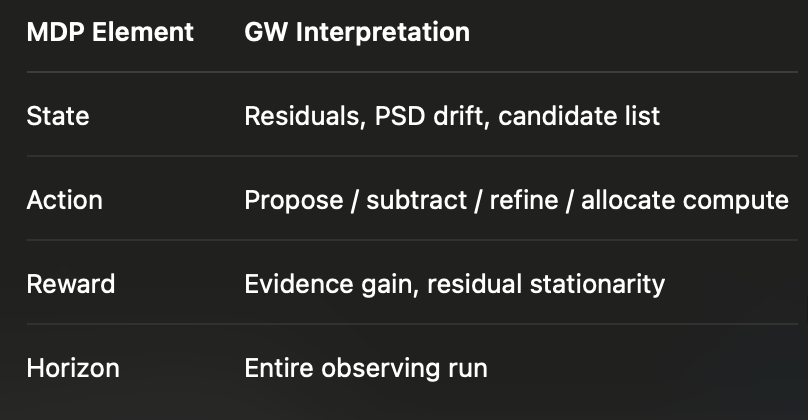
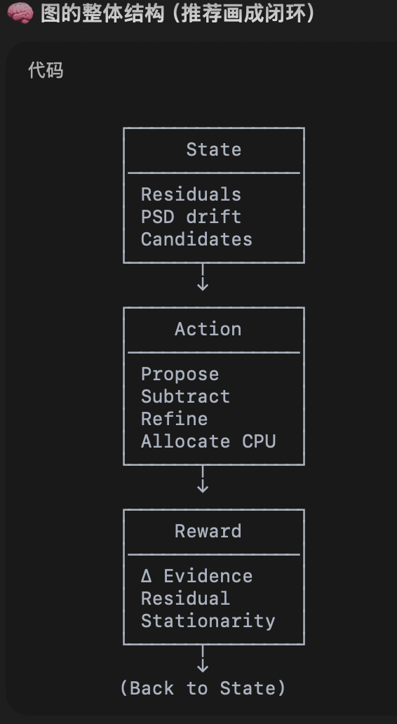
| MDP Element | GW Interpretation |
|---|---|
| State | Residuals, PSD drift, candidate list |
| Action | Propose/subtract/refine/allocate compute |
| Reward | Evidence gain, residual stationarity |
| Horizon | Entire observing run |
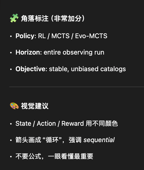
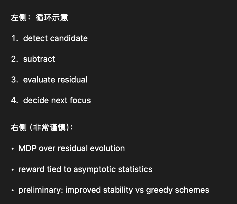
A trajectory tree of global-fitting decisions over time
Nodes: residual states
Edges: modeling actions
(HW+, in preparation)
Global fitting as a Markov Decision Process (MDP)

GW Data Analysis as a Markov Decision Process
Many GW pipelines already define an MDP — implicitly and inconsistently.
“Once you phrase the problem this way,
RL and MCTS are not exotic — they are obvious.”

Open Questions for the Community
- What is the right reward for discovery?
- Should we train ensembles instead of curating them?
- When does adaptivity beat optimality?
for _ in range(num_of_audiences):
    print('Thank you for your attention! 🙏')
Call for Speakers - MLA F2F @ March LVK 2026 (Pisa)
Just a gentle reminder that we’re collecting contributions for the Machine Learning Algorithms (MLA) section!
- 🔗 MLA Wiki: https://wiki.ligo.org/MLA/WebHome
- 🔗 Mattermost channel