


He Wang PRO
Knowledge increases by sharing but not by saving.
2026/01/27 | Flash Talk
GWFREERIDE: Carving the AI Gradient in Gravitational-Wave Astronomy
2026/01/23 · Flash Talk
GWFREERIDE: Carving the AI Gradient in Gravitational-Wave Astronomy
Adaptive trajectory, not a single optimum
Upcoming challenges such as MLGWSC2, currently at the proposal stage, provide a new testbed for exploring machine-learning–based approaches to gravitational-wave analysis. In this flash talk, I briefly introduce my core ideas and experience using evolutionary algorithms, Evo-MCTS, and reinforcement learning as adaptive search and optimization tools. I outline key methodological insights and discuss how these ideas may inform future GW analysis tasks, including potential applications to LISA.
才翻到上面看到有人现场拍照 [破涕为笑],随手分享一下
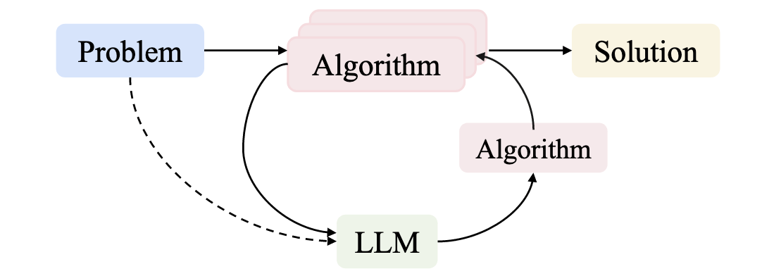
The LLM does not predict answers — it reshapes how we search for algorithms.
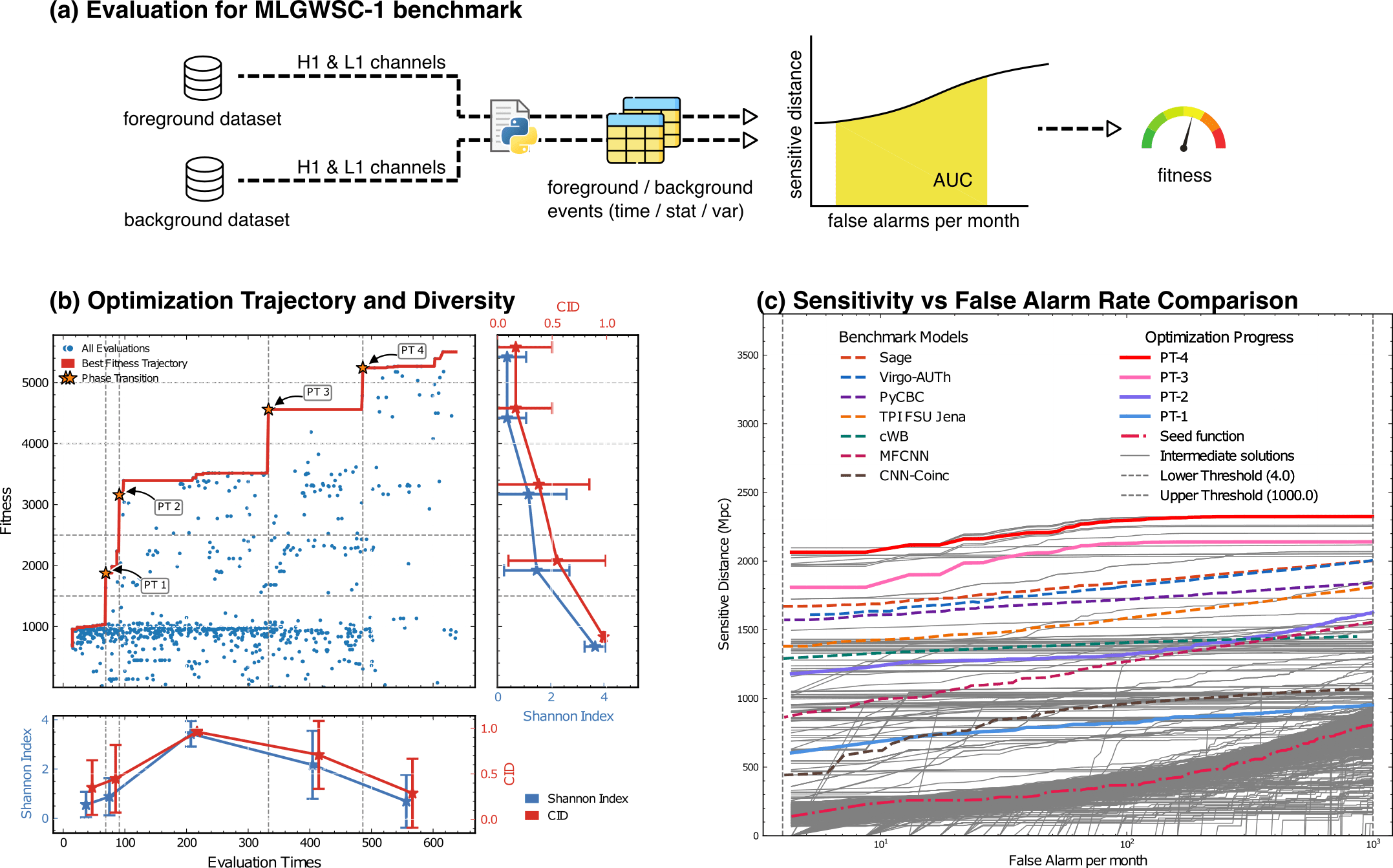
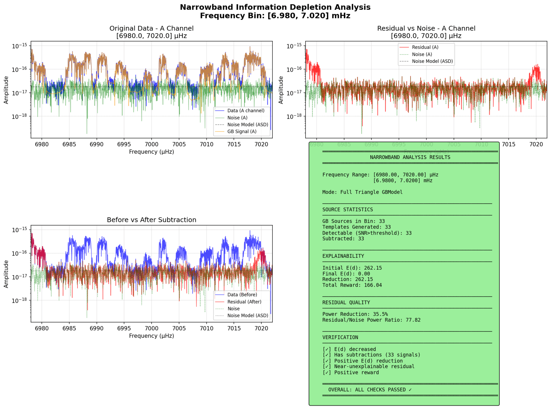
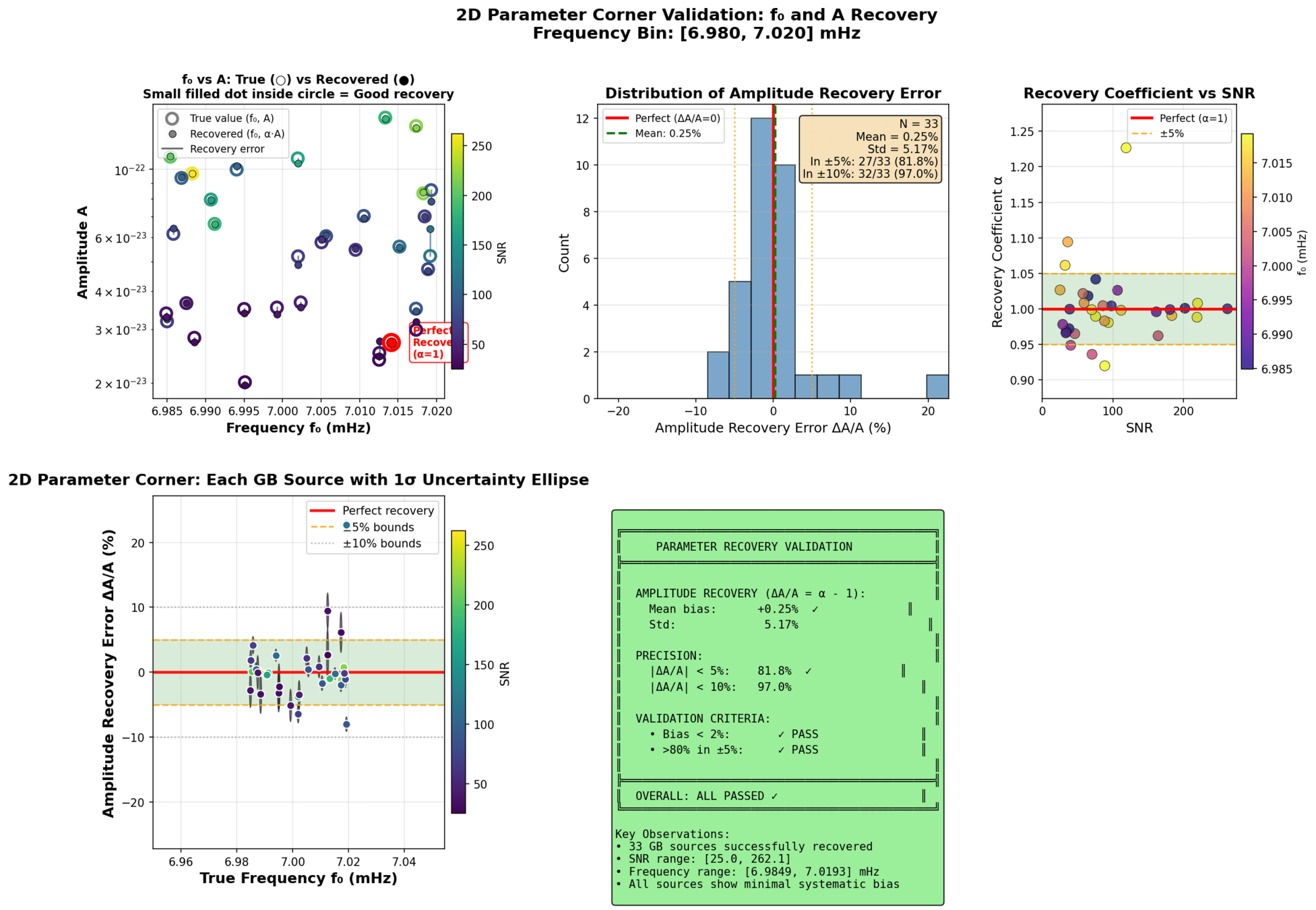
Evaluation for MLGWSC-1 benchmark
LLMs act as policies over algorithms, not predictors of data.
Concept
Mechanism
problem → algorithm
data → algorithm → reward
↺ LLM-guided algorithm updates
from problem-solving to algorithm discovery
HW, LZ. arXiv:2508.03661 [cs.AI]
The LLM does not predict answers — it reshapes how we search for algorithms.
external_knowledge
(constraint)
PyCBC (linear-core)
cWB (nonlinear-core)
Simple filters (non-linear)
CNN-like (highly non-linear)
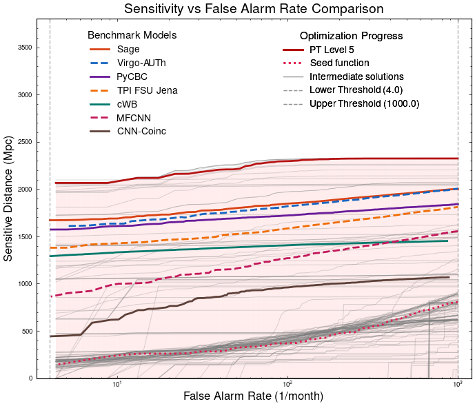
Benchmarking against state-of-the-art methods
Evaluation for MLGWSC-1 benchmark
LLM as designer
arXiv:2410.14716 [cs.LG]
HW, LZ. arXiv:2508.03661 [cs.AI]
LLMs act as adaptive policy priors over algorithmic decisions.
The LLM does not predict answers — it shapes the search process itself.
LLM proposes moves, not outputs
Search history becomes reusable knowledge
Algorithm behavior evolves, not just parameters
What changed?
LLMs do not predict waveforms or labels
LLMs propose actions that guide the search
Evaluations (fitness/likelihood) become reusable memory
Search trajectories matter more than isolated optima.
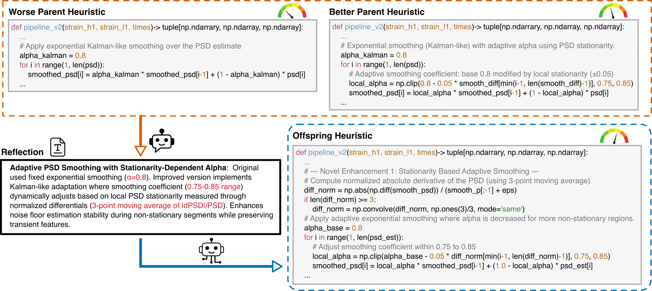
LLM-Driven Algorithmic Evolution Through Reflective Code Synthesis.
HW, LZ. arXiv:2508.03661 [cs.AI]
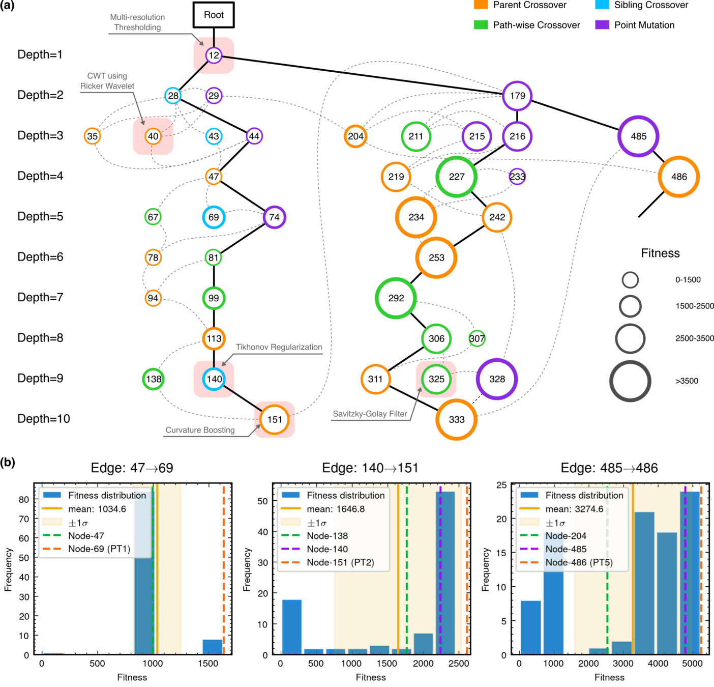
Monte Carlo Tree Search (MCTS) Algorithmic Evolution Pathway
What changed?
LLMs propose actions that guide the search
Evaluations (fitness/likelihood/...) become reusable memory
Search trajectories matter more than isolated optima.
The LLM does not predict answers — it reshapes how we search for algorithms.
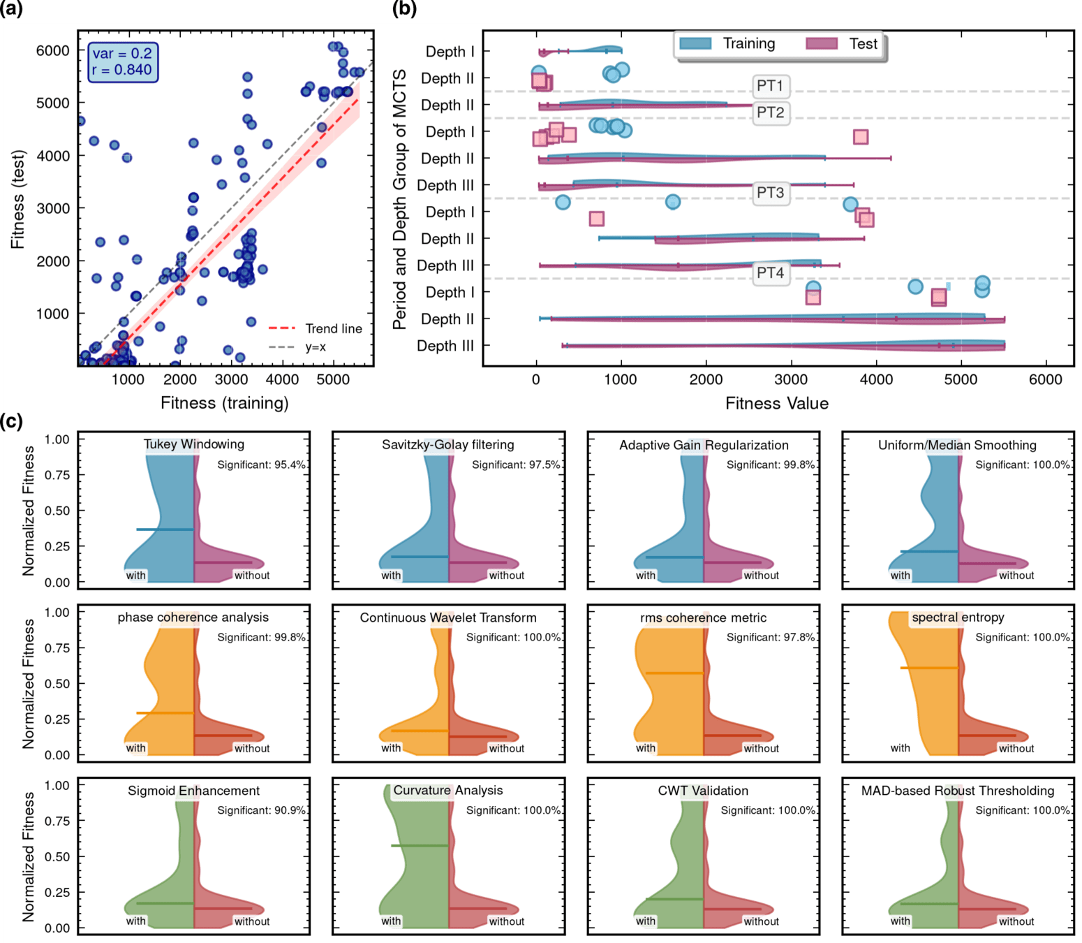
Algorithmic Component Impact Analysis.
import numpy as np
import scipy.signal as signal
from scipy.signal.windows import tukey
from scipy.signal import savgol_filter

def pipeline_v2(strain_h1: np.ndarray, strain_l1: np.ndarray, times: np.ndarray) -> tuple[np.ndarray, np.ndarray, np.ndarray]:
    """
    The pipeline function processes gravitational wave data from the H1 and L1 detectors to identify potential gravitational wave signals.
    It takes strain_h1 and strain_l1 numpy arrays containing detector data, and times array with corresponding time points.
    The function returns a tuple of three numpy arrays: peak_times containing GPS times of identified events,
    peak_heights with significance values of each peak, and peak_deltat showing time window uncertainty for each peak.
    """
    eps = np.finfo(float).tiny
    dt = times[1] - times[0]
    fs = 1.0 / dt
    # Base spectrogram parameters
    base_nperseg = 256
    base_noverlap = base_nperseg // 2
    medfilt_kernel = 101       # odd kernel size for robust detrending
    uncertainty_window = 5     # half-window for local timing uncertainty

    # -------------------- Stage 1: Robust Baseline Detrending --------------------
    # Remove long-term trends using a median filter for each channel.
    detrended_h1 = strain_h1 - signal.medfilt(strain_h1, kernel_size=medfilt_kernel)
    detrended_l1 = strain_l1 - signal.medfilt(strain_l1, kernel_size=medfilt_kernel)

    # -------------------- Stage 2: Adaptive Whitening with Enhanced PSD Smoothing --------------------
    def adaptive_whitening(strain: np.ndarray) -> np.ndarray:
        # Center the signal.
        centered = strain - np.mean(strain)
        n_samples = len(centered)
        # Adaptive window length: between 5 and 30 seconds
        win_length_sec = np.clip(n_samples / fs / 20, 5, 30)
        nperseg_adapt = int(win_length_sec * fs)
        nperseg_adapt = max(10, min(nperseg_adapt, n_samples))

        # Create a Tukey window with 75% overlap.
        tukey_alpha = 0.25
        win = tukey(nperseg_adapt, alpha=tukey_alpha)
        noverlap_adapt = int(nperseg_adapt * 0.75)
        if noverlap_adapt >= nperseg_adapt:
            noverlap_adapt = nperseg_adapt - 1

        # Estimate the power spectral density (PSD) using Welch's method.
        freqs, psd = signal.welch(centered, fs=fs, nperseg=nperseg_adapt,
                                  noverlap=noverlap_adapt, window=win, detrend='constant')
        psd = np.maximum(psd, eps)

        # Compute relative differences for PSD stationarity measure.
        diff_arr = np.abs(np.diff(psd)) / (psd[:-1] + eps)
        # Smooth the derivative with a moving average.
        if len(diff_arr) >= 3:
            smooth_diff = np.convolve(diff_arr, np.ones(3)/3, mode='same')
        else:
            smooth_diff = diff_arr

        # Exponential smoothing (Kalman-like) with adaptive alpha using PSD stationarity.
        smoothed_psd = np.copy(psd)
        for i in range(1, len(psd)):
            # Adaptive smoothing coefficient: base 0.8 modified by local stationarity (±0.05)
            local_alpha = np.clip(0.8 - 0.05 * smooth_diff[min(i-1, len(smooth_diff)-1)], 0.75, 0.85)
            smoothed_psd[i] = local_alpha * smoothed_psd[i-1] + (1 - local_alpha) * psd[i]

        # Compute Tikhonov regularization gain based on deviation from median PSD.
        noise_baseline = np.median(smoothed_psd)
        raw_gain = (smoothed_psd / (noise_baseline + eps)) - 1.0

        # Compute a causal-like gradient using the Savitzky-Golay filter.
        win_len = 11 if len(smoothed_psd) >= 11 else ((len(smoothed_psd)//2)*2+1)
        polyorder = 2 if win_len > 2 else 1
        delta_freq = np.mean(np.diff(freqs))
        grad_psd = savgol_filter(smoothed_psd, win_len, polyorder, deriv=1, delta=delta_freq, mode='interp')

        # Nonlinear scaling via sigmoid to enhance gradient differences.
        sigmoid = lambda x: 1.0 / (1.0 + np.exp(-x))
        scaling_factor = 1.0 + 2.0 * sigmoid(np.abs(grad_psd) / (np.median(smoothed_psd) + eps))

        # Compute adaptive gain factors with nonlinear scaling.
        gain = 1.0 - np.exp(-0.5 * scaling_factor * raw_gain)
        gain = np.clip(gain, -8.0, 8.0)

        # FFT-based whitening: interpolate gain and PSD onto FFT frequency bins.
        signal_fft = np.fft.rfft(centered)
        freq_bins = np.fft.rfftfreq(n_samples, d=dt)
        interp_gain = np.interp(freq_bins, freqs, gain, left=gain[0], right=gain[-1])
        interp_psd = np.interp(freq_bins, freqs, smoothed_psd, left=smoothed_psd[0], right=smoothed_psd[-1])
        denom = np.sqrt(interp_psd) * (np.abs(interp_gain) + eps)
        denom = np.maximum(denom, eps)
        white_fft = signal_fft / denom
        whitened = np.fft.irfft(white_fft, n=n_samples)
        return whitened

    # Whiten H1 and L1 channels using the adapted method.
    white_h1 = adaptive_whitening(detrended_h1)
    white_l1 = adaptive_whitening(detrended_l1)

    # -------------------- Stage 3: Coherent Time-Frequency Metric with Frequency-Conditioned Regularization --------------------
    def compute_coherent_metric(w1: np.ndarray, w2: np.ndarray) -> tuple[np.ndarray, np.ndarray]:
        # Compute complex spectrograms preserving phase information.
        f1, t_spec, Sxx1 = signal.spectrogram(w1, fs=fs, nperseg=base_nperseg,
                                              noverlap=base_noverlap, mode='complex', detrend=False)
        f2, t_spec2, Sxx2 = signal.spectrogram(w2, fs=fs, nperseg=base_nperseg,
                                               noverlap=base_noverlap, mode='complex', detrend=False)
        # Ensure common time axis length.
        common_len = min(len(t_spec), len(t_spec2))
        t_spec = t_spec[:common_len]
        Sxx1 = Sxx1[:, :common_len]
        Sxx2 = Sxx2[:, :common_len]

        # Compute phase differences and coherence between detectors.
        phase_diff = np.angle(Sxx1) - np.angle(Sxx2)
        phase_coherence = np.abs(np.cos(phase_diff))

        # Estimate median PSD per frequency bin from the spectrograms.
        psd1 = np.median(np.abs(Sxx1)**2, axis=1)
        psd2 = np.median(np.abs(Sxx2)**2, axis=1)

        # Frequency-conditioned regularization gain (reflection-guided).
        lambda_f = 0.5 * ((np.median(psd1) / (psd1 + eps)) + (np.median(psd2) / (psd2 + eps)))
        lambda_f = np.clip(lambda_f, 1e-4, 1e-2)
        # Regularization denominator integrating detector PSDs and lambda.
        reg_denom = (psd1[:, None] + psd2[:, None] + lambda_f[:, None] + eps)

        # Weighted phase coherence that balances phase alignment with noise levels.
        weighted_comp = phase_coherence / reg_denom

        # Compute axial (frequency) second derivatives as curvature estimates.
        d2_coh = np.gradient(np.gradient(phase_coherence, axis=0), axis=0)
        avg_curvature = np.mean(np.abs(d2_coh), axis=0)

        # Nonlinear activation boost using tanh for regions of high curvature.
        nonlinear_boost = np.tanh(5 * avg_curvature)
        linear_boost = 1.0 + 0.1 * avg_curvature

        # Cross-detector synergy: weight derived from global median consistency.
        novel_weight = np.mean((np.median(psd1) + np.median(psd2)) / (psd1[:, None] + psd2[:, None] + eps), axis=0)

        # Integrated time-frequency metric combining all enhancements.
        tf_metric = np.sum(weighted_comp * linear_boost * (1.0 + nonlinear_boost), axis=0) * novel_weight

        # Adjust the spectrogram time axis to account for window delay.
        metric_times = t_spec + times[0] + (base_nperseg / 2) / fs
        return tf_metric, metric_times

    tf_metric, metric_times = compute_coherent_metric(white_h1, white_l1)

    # -------------------- Stage 4: Multi-Resolution Thresholding with Octave-Spaced Dyadic Wavelet Validation --------------------
    def multi_resolution_thresholding(metric: np.ndarray, times_arr: np.ndarray) -> tuple[np.ndarray, np.ndarray, np.ndarray]:
        # Robust background estimation with median and MAD.
        bg_level = np.median(metric)
        mad_val = np.median(np.abs(metric - bg_level))
        robust_std = 1.4826 * mad_val
        threshold = bg_level + 1.5 * robust_std

        # Identify candidate peaks using prominence and minimum distance criteria.
        peaks, _ = signal.find_peaks(metric, height=threshold, distance=2, prominence=0.8 * robust_std)
        if peaks.size == 0:
            return np.array([]), np.array([]), np.array([])

        # Local uncertainty estimation using a Gaussian-weighted convolution.
        win_range = np.arange(-uncertainty_window, uncertainty_window + 1)
        sigma = uncertainty_window / 2.5
        gauss_kernel = np.exp(-0.5 * (win_range / sigma) ** 2)
        gauss_kernel /= np.sum(gauss_kernel)
        weighted_mean = np.convolve(metric, gauss_kernel, mode='same')
        weighted_sq = np.convolve(metric ** 2, gauss_kernel, mode='same')
        variances = np.maximum(weighted_sq - weighted_mean ** 2, 0.0)
        uncertainties = np.sqrt(variances)
        uncertainties = np.maximum(uncertainties, 0.01)

        valid_times = []
        valid_heights = []
        valid_uncerts = []
        n_metric = len(metric)

        # Compute a simple second derivative for local curvature checking.
        if n_metric > 2:
            second_deriv = np.diff(metric, n=2)
            second_deriv = np.pad(second_deriv, (1, 1), mode='edge')
        else:
            second_deriv = np.zeros_like(metric)

        # Use octave-spaced scales (dyadic wavelet validation) to validate peak significance.
        widths = np.arange(1, 9)  # approximate scales 1 to 8
        for peak in peaks:
            # Skip peaks lacking sufficient negative curvature.
            if second_deriv[peak] > -0.1 * robust_std:
                continue
            local_start = max(0, peak - uncertainty_window)
            local_end = min(n_metric, peak + uncertainty_window + 1)
            local_segment = metric[local_start:local_end]
            if len(local_segment) < 3:
                continue
            try:
                cwt_coeff = signal.cwt(local_segment, signal.ricker, widths)
            except Exception:
                continue
            max_coeff = np.max(np.abs(cwt_coeff))
            # Threshold for validating the candidate using local MAD.
            cwt_thresh = mad_val * np.sqrt(2 * np.log(len(local_segment) + eps))
            if max_coeff >= cwt_thresh:
                valid_times.append(times_arr[peak])
                valid_heights.append(metric[peak])
                valid_uncerts.append(uncertainties[peak])

        if len(valid_times) == 0:
            return np.array([]), np.array([]), np.array([])
        return np.array(valid_times), np.array(valid_heights), np.array(valid_uncerts)

    peak_times, peak_heights, peak_deltat = multi_resolution_thresholding(tf_metric, metric_times)
return peak_times, peak_heights, peak_deltatPT Level 5
Integrated Architecture Validation
Contributions of knowledge synthesis
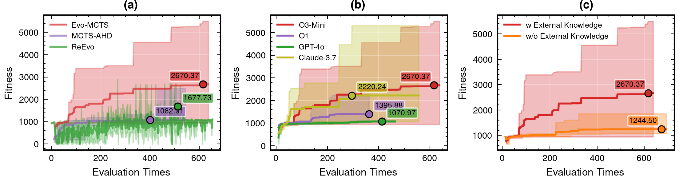
LLM Model Selection and Robustness Analysis
o3-mini-medium
o1-2024-12-17
gpt-4o-2024-11-20
claude-3-7-sonnet-20250219-thinking
59.1%
115%
AI and Cosmology: From Computational Tools to Scientific Discovery
Contributions of knowledge synthesis
59.1%
115%
59.1%
### External Knowledge Integration
1. **Non-linear** Processing Core Concepts:
- Signal Transformation:
* Non-linear vs linear decomposition
* Adaptive threshold mechanisms
* Multi-scale analysis
- Feature Extraction:
* Phase space reconstruction
* Topological data analysis
* Wavelet-based detection
- Statistical Analysis:
* Robust estimators
* Non-Gaussian processes
* Higher-order statistics
2. Implementation Principles:
- Prioritize adaptive over fixed parameters
- Consider local vs global characteristics
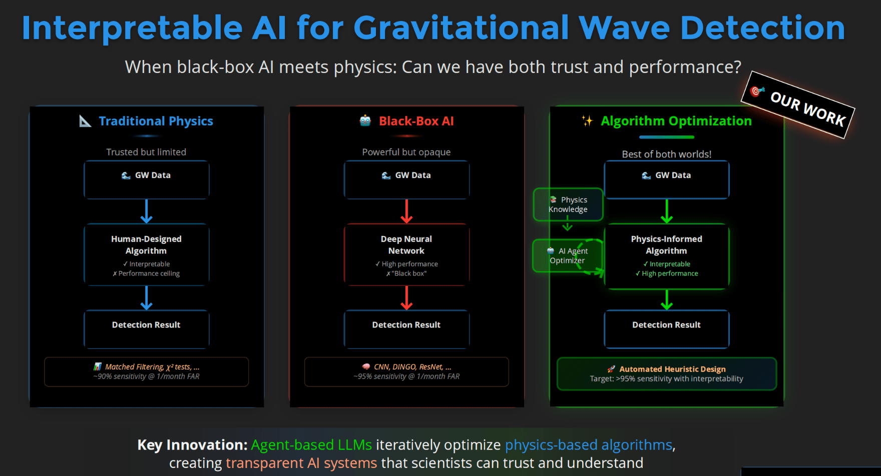
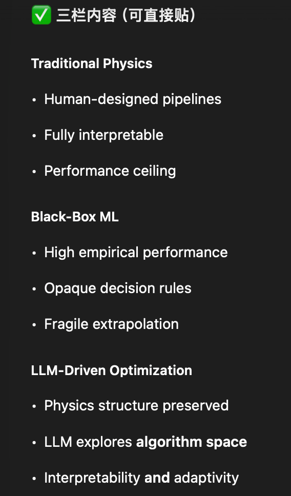
- Balance computational cost with accuracy✓ Fully interpretable
✗ Performance ceiling
Human-designed pipelines
Fixed heuristics
Examples:
Matched filtering
χ² tests
✓ High performance
✗ Opaque decisions
End-to-end prediction
Model-centric learning
Examples:
CNNs, DINGO
Algorithms as search objects
Physics-informed objectives
Example:
Evo-MCTS (this work)
AlphaEvolve
Scientific discovery requires interpretability — not just performance.
AI should help us understand why an algorithm works — not just output an answer.
PyCBC (linear-core)
cWB (nonlinear-core)
Simple filters (non-linear)
CNN-like (highly non-linear)
Benchmarking against state-of-the-art methods
(MLGWSC1)
HW, LZ. arXiv:2508.03661 [cs.AI]
Interpretable AI Approach
The best of both worlds
Input
Physics-Informed
Algorithm
(High interpretability)
Output
Example: Evo-MCTS, AlphaEvolve
AI Model
Physics
Knowledge
Traditional Physics Approach
Input
Human-Designed Algorithm
(Based on human insight)
Output
Example: Matched Filtering, linear regression
Black-Box AI Approach
Input
AI Model
(Low interpretability)
Output
Examples: CNN, AlphaGo, DINGO
Data/
Experience
Data/
Experience
🎯 OUR WORK
Scientific discovery requires interpretability, not just performance.
Scientific discovery requires interpretability — not just performance.
AI should help us understand why an algorithm works — not just output an answer.
Any algorithm design problem can be seen as an optimization problem
vs
LLMs as agents that optimize physics-based algorithms
A new axis: adaptivity over algorithm design
LLMs allow us to search over algorithms, not just over parameters.
✓ Fully interpretable
✗ Performance ceiling
Human-designed pipelines
Fixed heuristics
Examples:
Matched filtering
χ² tests
✓ High performance
✗ Opaque decisions
End-to-end prediction
Model-centric learning
Examples:
CNNs, DINGO
✓ Interpretable
✓ High performance
Algorithms as search objects
Physics-informed objectives
Example:
Evo-MCTS (this work)
Interpretable AI Approach
The best of both worlds
Input
Physics-Informed
Algorithm
(High interpretability)
Output
Example: Evo-MCTS, AlphaEvolve
AI Model
Physics
Knowledge
Traditional Physics Approach
Input
Human-Designed Algorithm
(Based on human insight)
Output
Example: Matched Filtering, linear regression
Black-Box AI Approach
Input
AI Model
(Low interpretability)
Output
Examples: CNN, AlphaGo, DINGO
Data/
Experience
Data/
Experience
🎯 OUR WORK
What do we think about AI for scientific discovery?
Scientific discovery requires interpretability, not just performance.
From single-pipeline performance to ensemble unbiasedness
We emphasize evaluating complementarity and ensemble behavior rather than single-pipeline superiority.
What LVK already does
GWTC catalogs rely on multiple independent pipelines
A candidate proceeds if any pipeline produces a confidence trigger
This already forms an implicit ensemble
Ensembling is already standard practice — just not explicitly analyzed.
The missing question
Each pipeline carries distinct inductive biases
(eg: duration, morphology, noise response, parameter coverage).
cWB
GstLAL
PyCBC
AI_1
AI_2
AI_3
AI_n
Is the ensemble unbiased?
LVK anchor pipelines
(selected)
Ensemble evaluation
MLGWSC-2 is under proposal development with active community input (e.g. Nitz, Dent, Messenger, ...).
Related works
“I don’t claim this is solved. I claim the framing matters.”
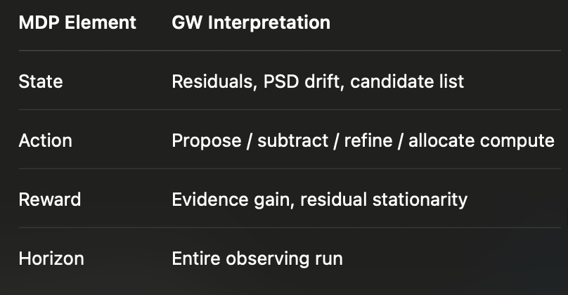
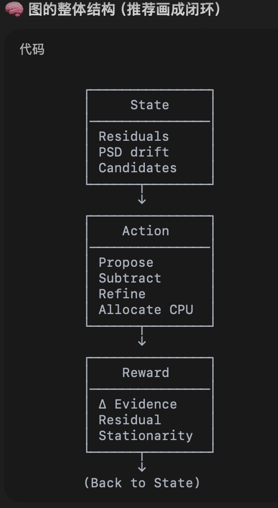
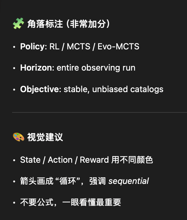
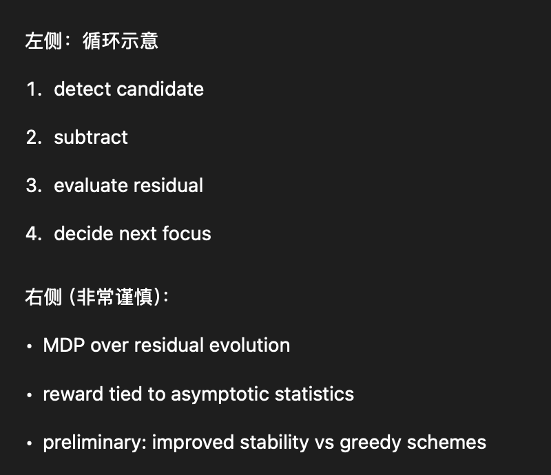
Global fitting is not a single inference — it is a long-horizon control problem.
preliminary
preliminary
MH Du+, arXiv:2505.16500 [gr-qc]
| MDP Element | GW Interpretation |
|---|---|
| State | Residuals, PSD drift, candidate list |
| Action | Propose/subtract/refine/allocate compute |
| Reward | Evidence gain, residual stationarity |
| Horizon | Entire observing run |
A trajectory tree of global-fitting decisions over time
Nodes: residual states
Edges: modeling actions
(HW+, in preparation)
Global fitting as a Markov Decision Process (MDP)
Many GW pipelines already define an MDP — implicitly and inconsistently.
“Once you phrase the problem this way,
RL and MCTS are not exotic — they are obvious.”
for _ in range(num_of_audiences):
    print('Thank you for your attention! 🙏')
Call for Speakers - MLA F2F @ March LVK 2026 (Pisa)
Just a gentle reminder that we’re collecting contributions for the Machine Learning Algorithms (MLA) section!
By He Wang
2026/01/27 | Flash Talk @GWFREERIDE | Abstract: Upcoming challenges such as MLGWSC2, currently at the proposal stage, provide a new testbed for exploring machine-learning–based approaches to gravitational-wave analysis. In this flash talk, I briefly introduce my core ideas and experience using evolutionary algorithms, Evo-MCTS, and reinforcement learning as adaptive search and optimization tools. I outline key methodological insights and discuss how these ideas may inform future GW analysis tasks, including potential applications to LISA.


