Matched-filtering Techniques
& Deep Neural Networks
—— Application for Gravitational-wave Astronomy



He Wang (王赫)
Institute of Theoretical Physics, CAS
Member of KAGRA collaboration
Apache MXNet Day, 10:01 AM PST on December 14\(^\text{th}\), 2020
Based on DOI: 10.1103/physrevd.101.104003

hewang@mail.bnu.edu.cn / hewang@itp.ac.cn
OVERVIEW
- Gravitational-wave (GW) Astronomy
- Challenges & Opportunities
- Motivation
- Matched-filtering Convolutional Neural Network (MFCNN)
- Lessons Learned

Gravitational Wave
from binary black hole merges
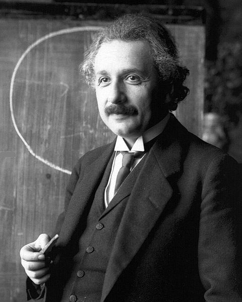
- 100 years from Einstein's prediction to the first LIGO-Virgo detection (GW150914) announcement in 2016.
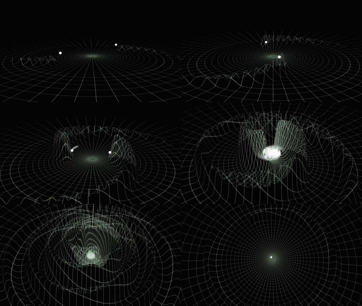
- General relativity: "Spacetime tells matter how to move, and matter tells spacetime how to curve."
- Time-varying quadrupolar mass distributions lead to propagating ripples in spacetime: GWs.
Gravitational-wave Astronomy
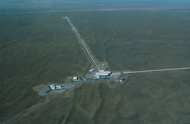
LIGO Hanford (H1)

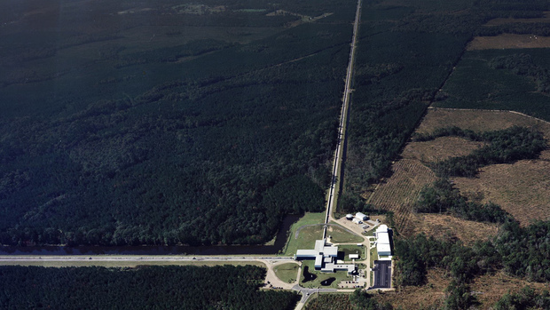
LIGO Livingston (L1)
KAGRA
- Advanced LIGO observing since 2015 (two detectors in US), joined by Virgo (Italy) in 2017 and KAGRA (Japan) in Japan in 2020.
- Best GW hunter in the range 10Hz-10kHz.

Challenges in GW Data Analysis
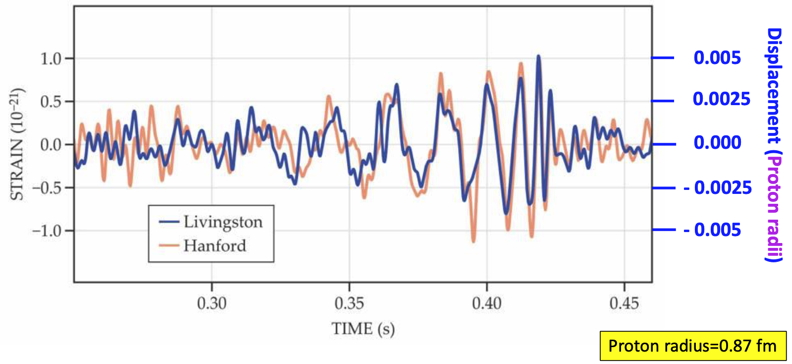
- Event GW150914
- On September 14th, 2015: GWs from two ~30 solar mass black holes (BHs), merging ~400Mpc from Earth (z~0.1), crossed the two LIGO detectors displacing their test masses by a small fraction of the radius of a proton.
- Measuring intervals must be smaller than 0.01 seconds.
Credit: LIGO

- Noise in the detector
- The actual data from the detector is shown in gray.
- The noise is much louder (~100x) than the expected signals
in red, green and blue. (BHs with spinning/non-spining and two neutron stars) - It's non-Gaussian and non-stationary that containing anomalous non-Gaussian transients, known as glitches.
Challenges in GW Data Analysis
Noise power spectral density (one-sided)
-
Matched-filtering Technique
- It is an optimal linear filter for weak signals buried in Gaussian and stationary noise \(n(t)\).
- Works by correlating a known signal model \(h(t)\) (template) with the data.
- Starting with data: \(d(t) = h(t) + n(t)\).
- Defining the matched-filtering SNR \(\rho(t)\):
where
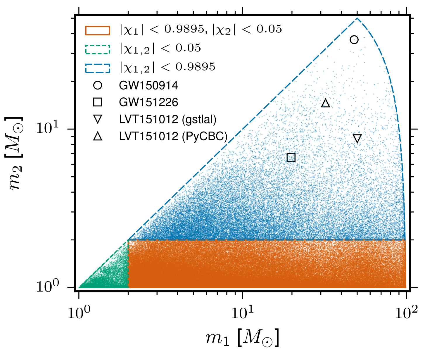
- The 4-D search parameter space in the first observation run covered by a template bank to circular binaries for which the spin of the systems is aligned (or antialigned) with the orbital angular momentum of the binary.
- ~250,000 template waveforms are used (computationally expansive).
The template that best matches GW150914 event
-
Phys.Rev.D 97 (2018) 4, 044039
- The first attempt
-
Phys.Rev.Lett 120 (2019) 14, 141103
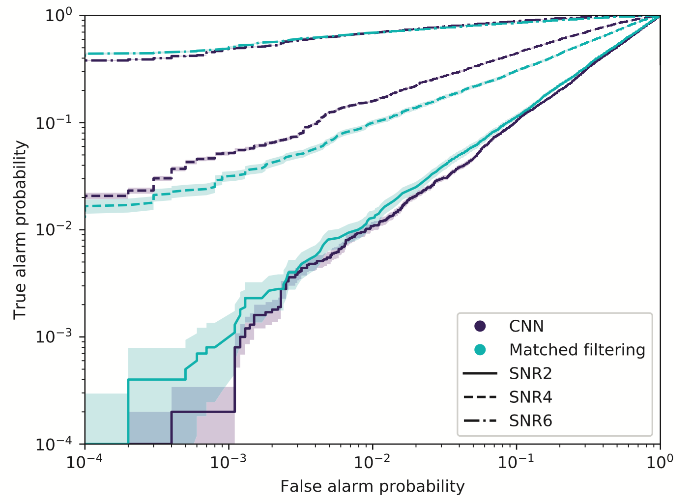
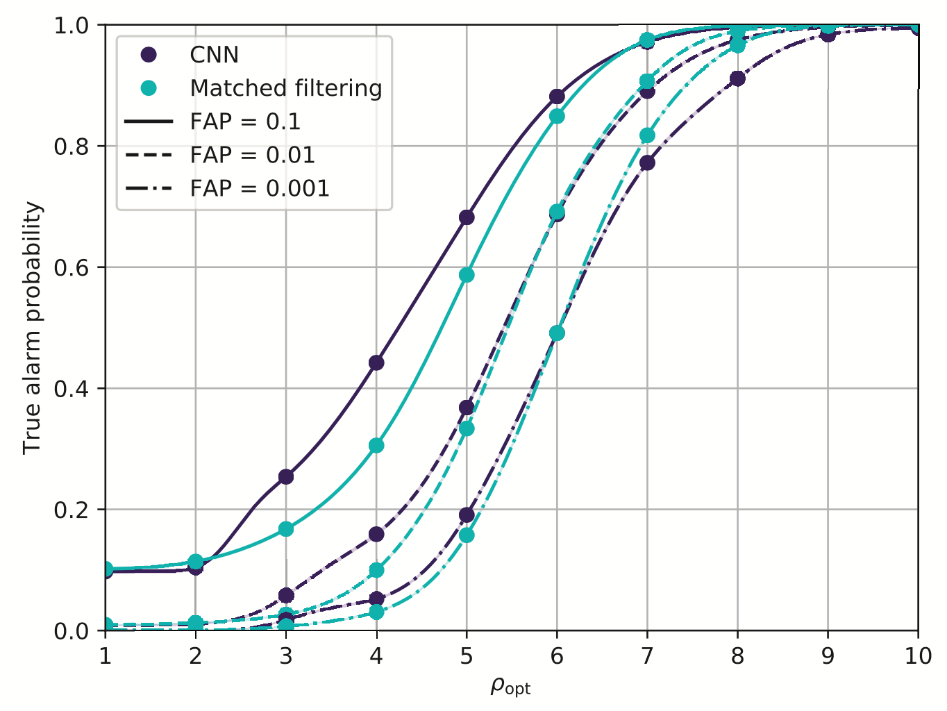
- Matched-filtering vs CNN
...
-
Phys.Rev.D 100 (2019) 6, 063015
- GW events for BBH
-
Phys.Rev.D 101 (2020) 10, 104003
- All GW events in O1/O2
Proof-of-principle studies
Production search studies
Milestones
More related works, see Survey4GWML (https://iphysresearch.github.io/Survey4GWML/)
- When machine & deep learning meets GW astronomy:
- Covering more parameter-space (Interpolation)
- Automatic generalization to new sources (Extrapolation)
-
Resilience to real non-Gaussian noise (Robustness)
-
Acceleration of existing pipelines (Speed, <0.1ms)
Opportunities in GW Data Analysis
Stimulated background noises
Attempts on Real LIGO Noise


A specific design of the architecture is needed.
Classification

Feature extraction
Convolutional neural network (ConvNet or CNN)
- CNNs always works pretty good on stimulated noises.
- However, when on real noises from LIGO, this approach does not work that well.
- It's too sensitive against the background + hard to find GW events)
Attempts on Real LIGO Noise
- CNNs always works pretty good on stimulated noises.
- However, when on real noises from LIGO, this approach does not work that well.
- It's too sensitive against the background + hard to find GW events)
A specific design of the architecture is needed.
Classification

Feature extraction


Convolutional neural network (ConvNet or CNN)
MFCNN
MFCNN
MFCNN
Motivation
Classification

Feature extraction
Convolutional neural network (ConvNet or CNN)
- With the closely related concepts between the templates and kernels , we attempt to address a question of:
Matched-filtering (cross-correlation with the templates) can be regarded as a convolutional layer with a set of predefined kernels.
>> Is it matched-filtering ?
>> Wait, It can be matched-filtering!
- In practice, we use matched filters as an essential component of feature extraction in the first part of the CNN for GW detection.
Matched-filtering CNNs (MFCNN)
\(S_n(|f|)\) is the one-sided average PSD of \(d(t)\)
(whitening)
where
Time domain
Frequency domain
(normalizing)
(matched-filtering)
- Transform matched-filtering method from frequency domain to time domain.
- The square of matched-filtering SNR for a given data \(d(t) = n(t)+h(t)\):
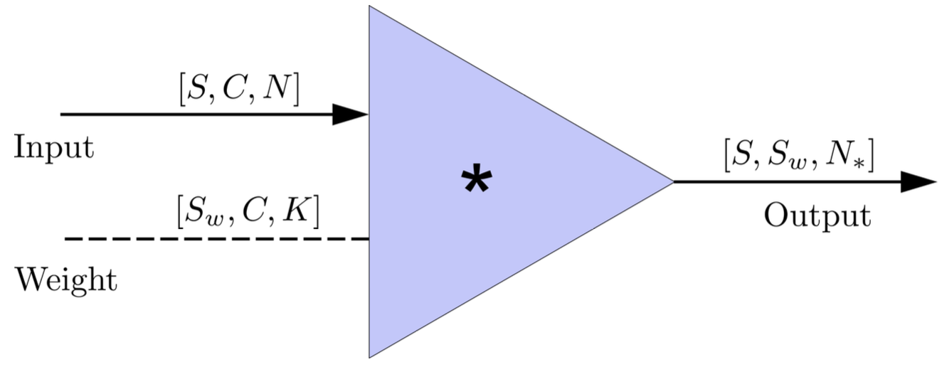
- In the 1-D convolution (\(*\)) on Apache MXNet, given input data with shape [batch size, channel, length] :
FYI: \(N_\ast = \lfloor(N-K+2P)/S\rfloor+1\)
(A schematic illustration for a unit of convolution layer)
Matched-filtering CNNs (MFCNN)
\(S_n(|f|)\) is the one-sided average PSD of \(d(t)\)
(whitening)
where
Time domain
Frequency domain
(normalizing)
(matched-filtering)
- Transform matched-filtering method from frequency domain to time domain.
- The square of matched-filtering SNR for a given data \(d(t) = n(t)+h(t)\):
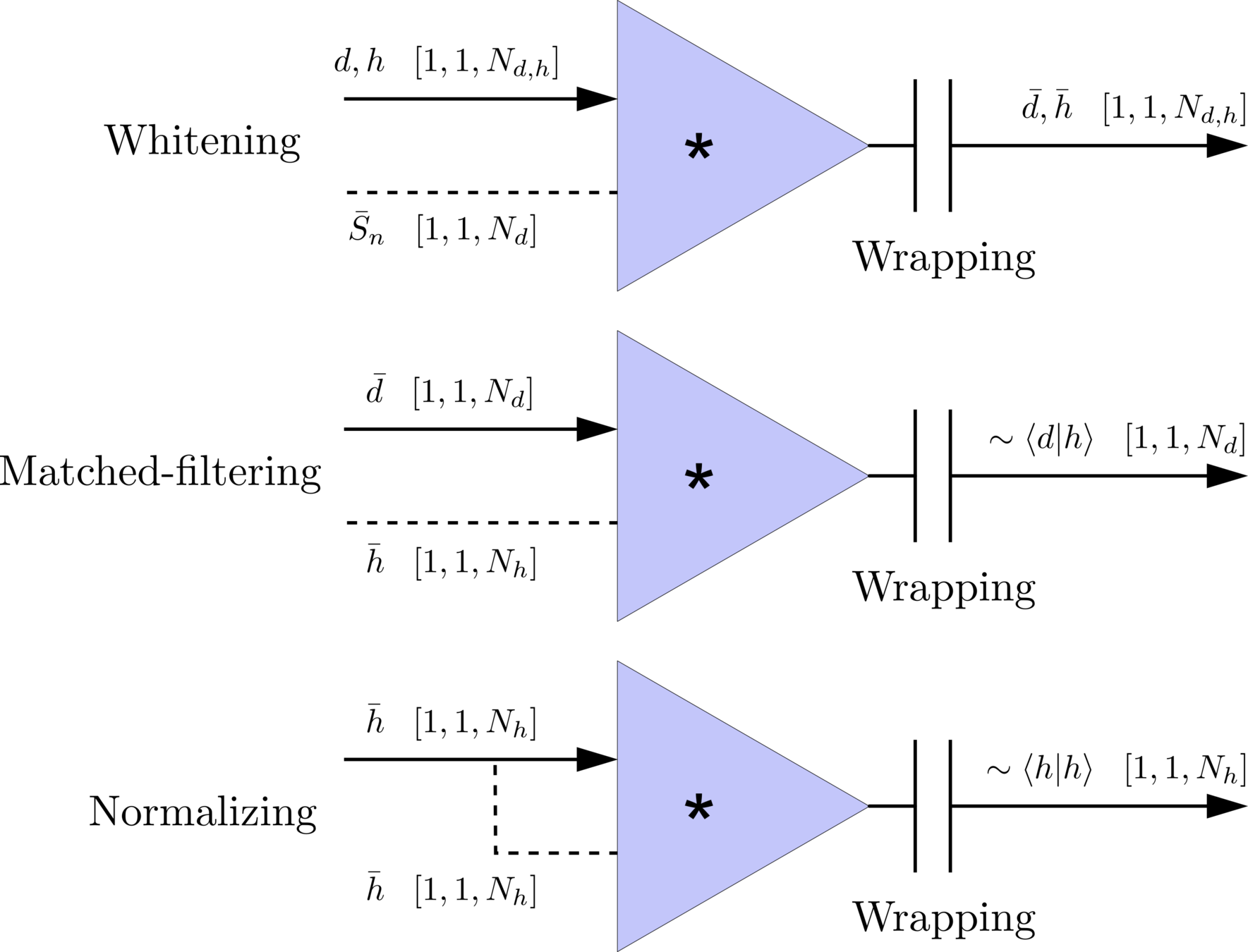


Apache MXNet Framework
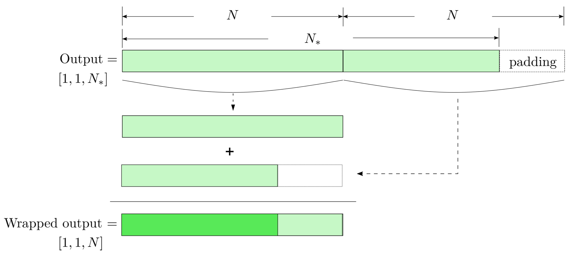
modulo-N circular convolution
Matched-filtering CNNs (MFCNN)
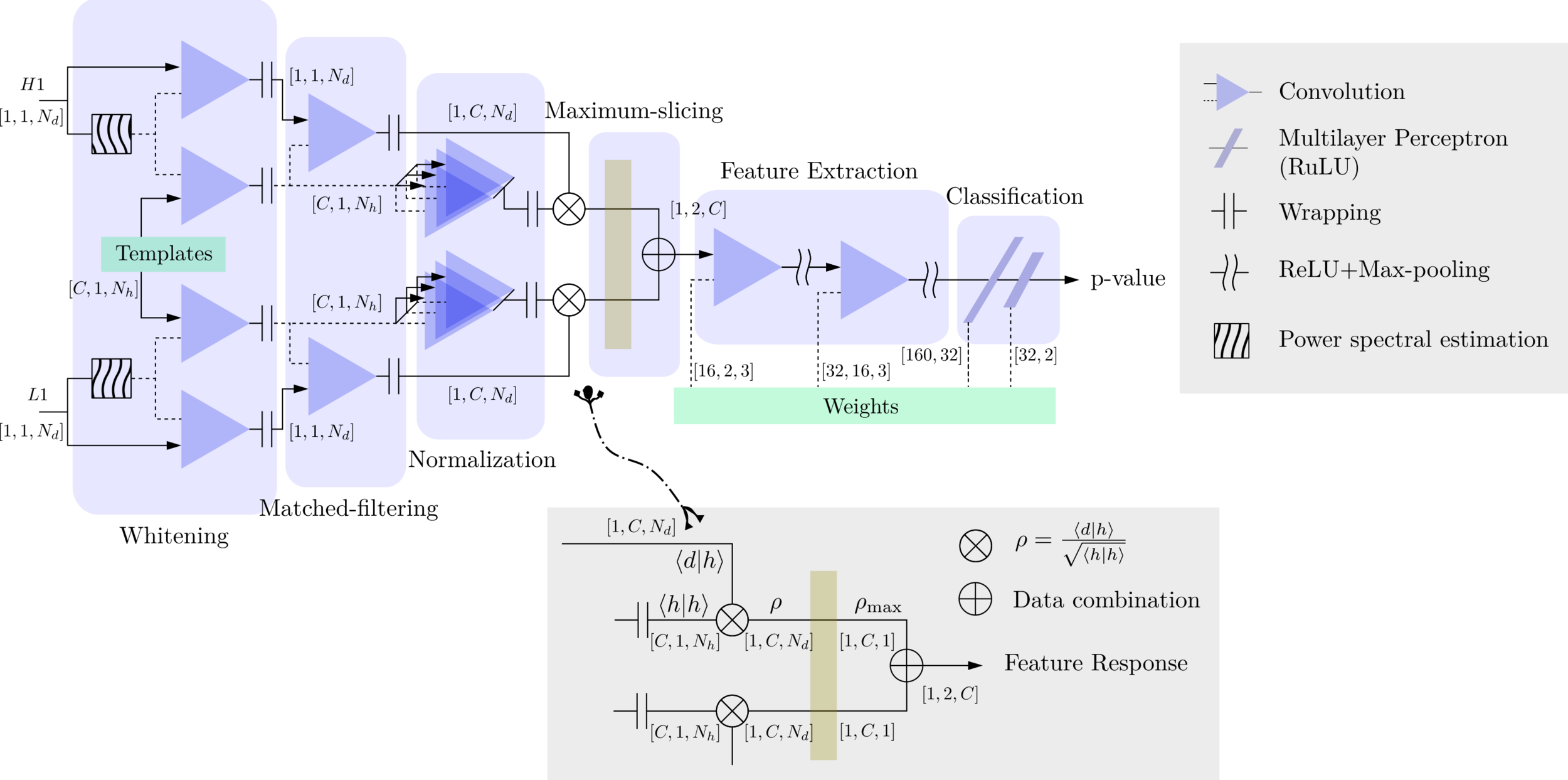
- The structure of MFCNN:
Input

Output
Matched-filtering CNNs (MFCNN)
Input
- The structure of MFCNN:
- In the meanwhile, we can obtain the optimal time \(N_0\) (relative to the input) of feature response of matching by recording the location of the maxima value corresponding to the optimal template \(C_0\).


Output
Matched-filtering CNNs (MFCNN)
- The structure of MFCNN:
Input
- In the meanwhile, we can obtain the optimal time \(N_0\) (relative to the input) of feature response of matching by recording the location of the maxima value corresponding to the optimal template \(C_0\).


Output
import mxnet as mx
from mxnet import nd, gluon
from loguru import logger

def MFCNN(fs, T, C, ctx, template_block, margin, learning_rate=0.003):
    logger.success('Loading MFCNN network!')
    net = gluon.nn.Sequential()
    with net.name_scope():
        net.add(MatchedFilteringLayer(mod=fs*T, fs=fs,
                                      template_H1=template_block[:,:1],
                                      template_L1=template_block[:,-1:]))
        net.add(CutHybridLayer(margin = margin))
        net.add(Conv2D(channels=16, kernel_size=(1, 3), activation='relu'))
        net.add(MaxPool2D(pool_size=(1, 4), strides=2))
        net.add(Conv2D(channels=32, kernel_size=(1, 3), activation='relu'))
        net.add(MaxPool2D(pool_size=(1, 4), strides=2))
        net.add(Flatten())
        net.add(Dense(32))
        net.add(Activation('relu'))
        net.add(Dense(2))
	# Initialize parameters of all layers
    net.initialize(mx.init.Xavier(magnitude=2.24), ctx=ctx, force_reinit=True)
    return net
The available codes: https://gist.github.com/iphysresearch/a00009c1eede565090dbd29b18ae982c
Lessons Learned
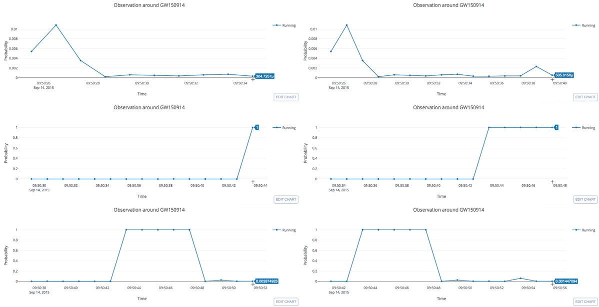
input
GW Data from GWOSC: https://www.gw-openscience.org/
This slide: https://slides.com/iphysresearch/apachemxnet_mfcnn
- Some benefits from MF-CNN architecture for GW detection:
- Simple configuration for GW data generation and almost no data pre-processing.
- It works on a non-stationary background.
- Easy parallel deployments, multiple detectors can benefit a lot from this design.
- Efficient searching with a fixed window.
- Dr. Chris Messenger (University of Glasgow):
“For me, it seems completely obvious that all data analysis will be ML in 5-10 years". - The main understanding of the algorithms for DL community:
- GW templates are used as likely known features for recognition.
- Generalization of both matched-filtering and neural networks.
- Linear filtering (i.e. matched-filtering) in signal processing can be rewritten as deep neural networks (i.e. CNNs).
- Rethinking the structure of neural networks? (data flow vs. weight flow)


Lessons Learned
input
- Some benefits from MF-CNN architecture for GW detection:
- Simple configuration for GW data generation and almost no data pre-processing.
- It works on a non-stationary background.
- Easy parallel deployments, multiple detectors can benefit a lot from this design.
- Efficient searching with a fixed window.
- Dr. Chris Messenger (University of Glasgow):
“For me, it seems completely obvious that all data analysis will be ML in 5-10 years". - The main understanding of the algorithms for DL community:
- GW templates are used as likely known features for recognition.
- Generalization of both matched-filtering and neural networks.
- Linear filtering (i.e. matched-filtering) in signal processing can be rewritten as deep neural networks (i.e. CNNs).
- Rethinking the structure of neural networks? (data flow vs. weight flow)


for _ in range(num_of_audiences):
    print('Thank you for your attention!')
Profile: iphysresearch.github.io/-he.wang/
Twitter: twitter.com/@Herb_hewang
GW Data from GWOSC: https://www.gw-openscience.org/
This slide: https://slides.com/iphysresearch/apachemxnet_mfcnn