


He Wang PRO
Knowledge increases by sharing but not by saving.
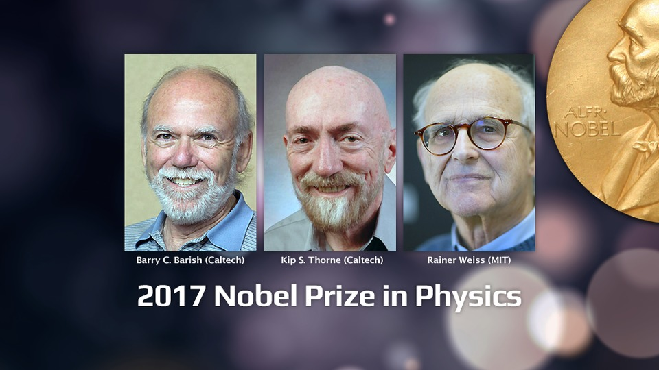
—— Application for Gravitational-wave Astronomy
He Wang (王赫)
Institute of Theoretical Physics, CAS
Member of KAGRA collaboration
Apache MXNet Day, 10:01 AM PST on December 14\(^\text{th}\), 2020
Based on DOI: 10.1103/physrevd.101.104003
hewang@mail.bnu.edu.cn / hewang@itp.ac.cn
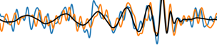
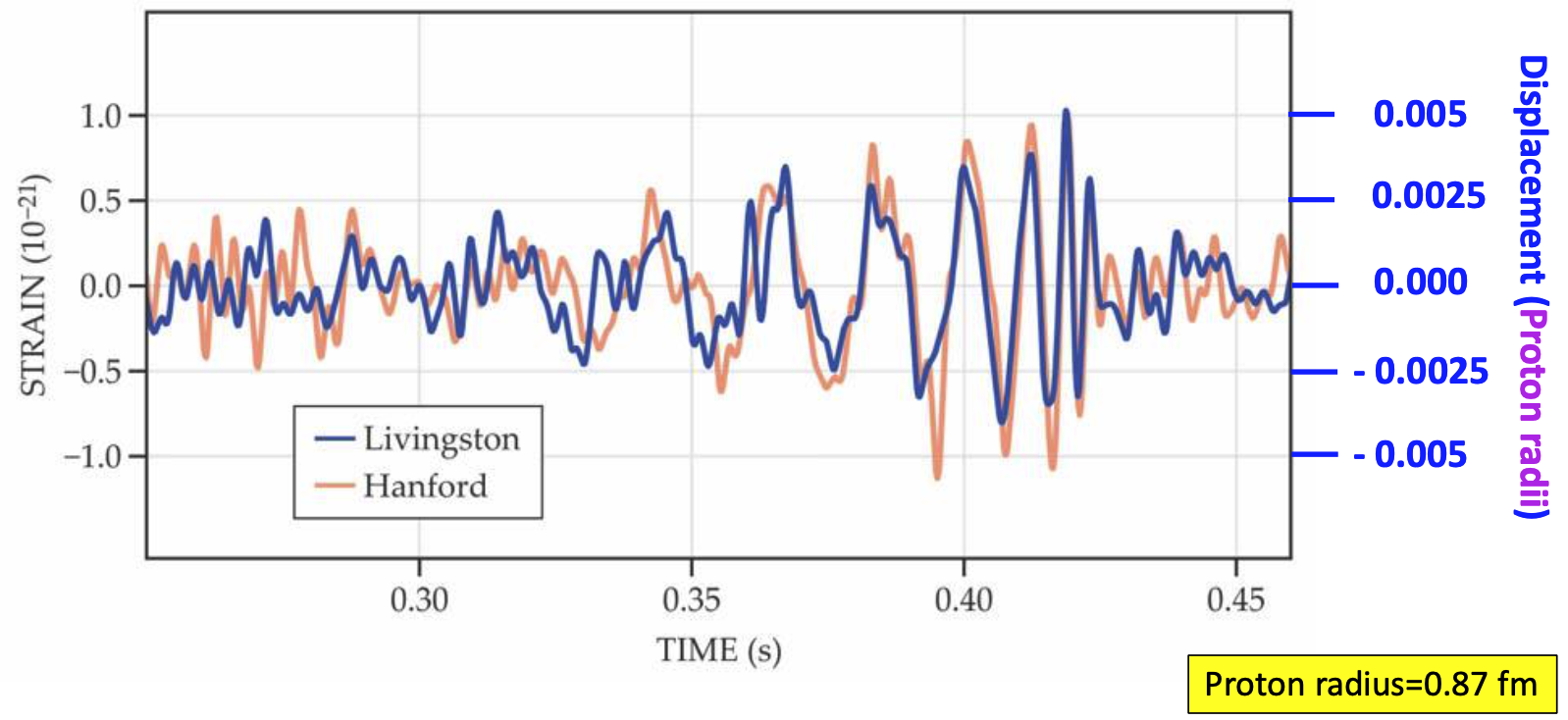
from binary black hole merges
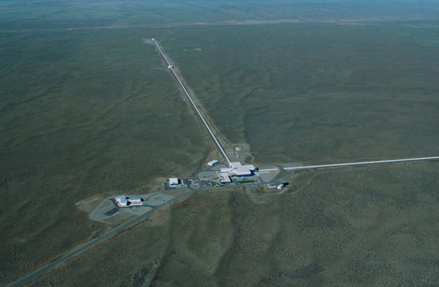
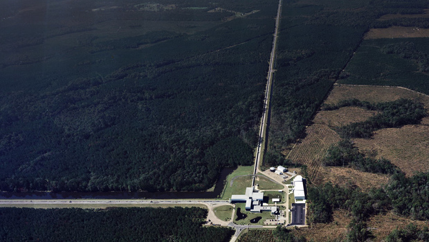
LIGO Hanford (H1)
LIGO Livingston (L1)
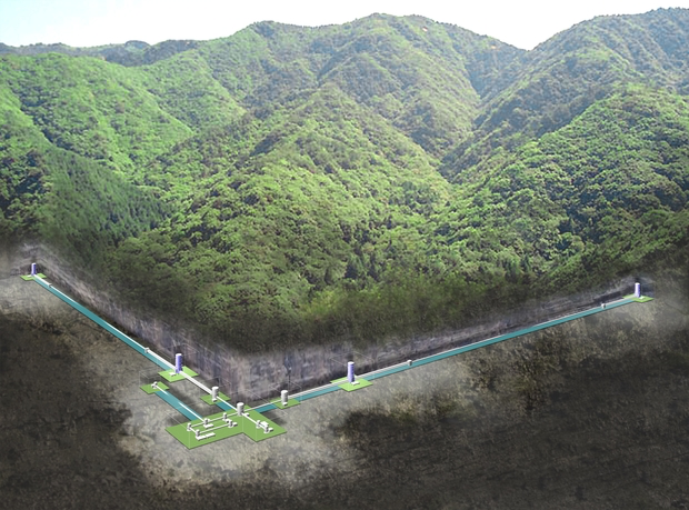
KAGRA
Credit: LIGO
Noise power spectral density (one-sided)
where
The template that best matches GW150914 event
...
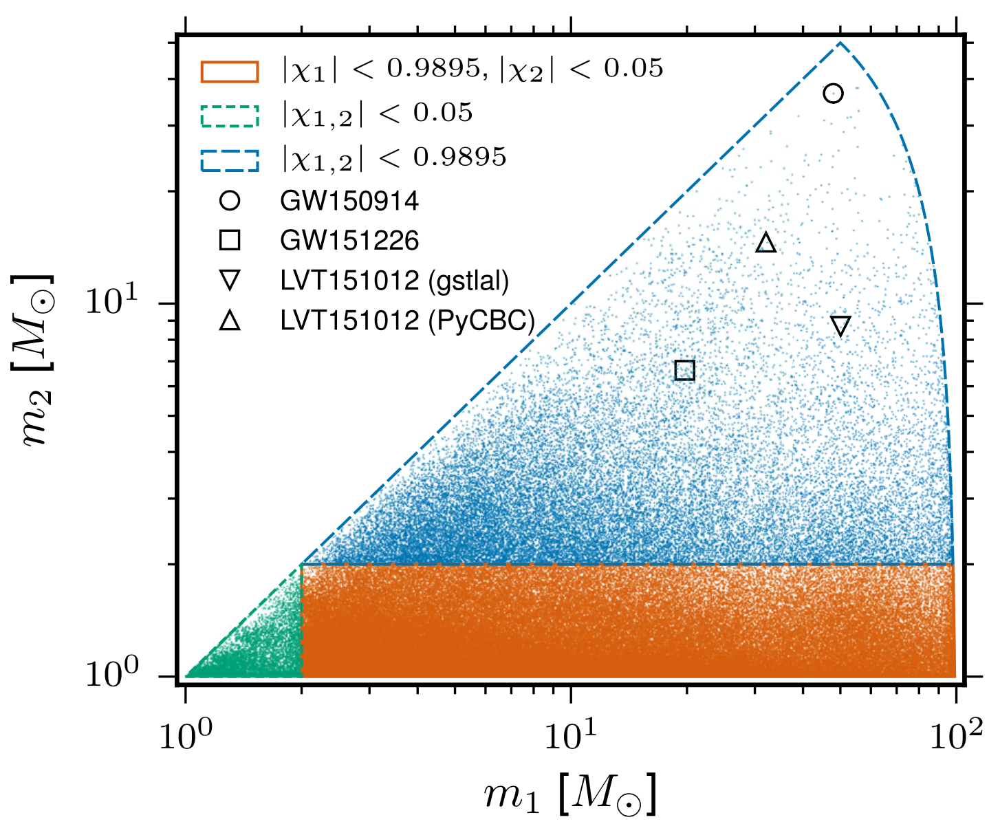
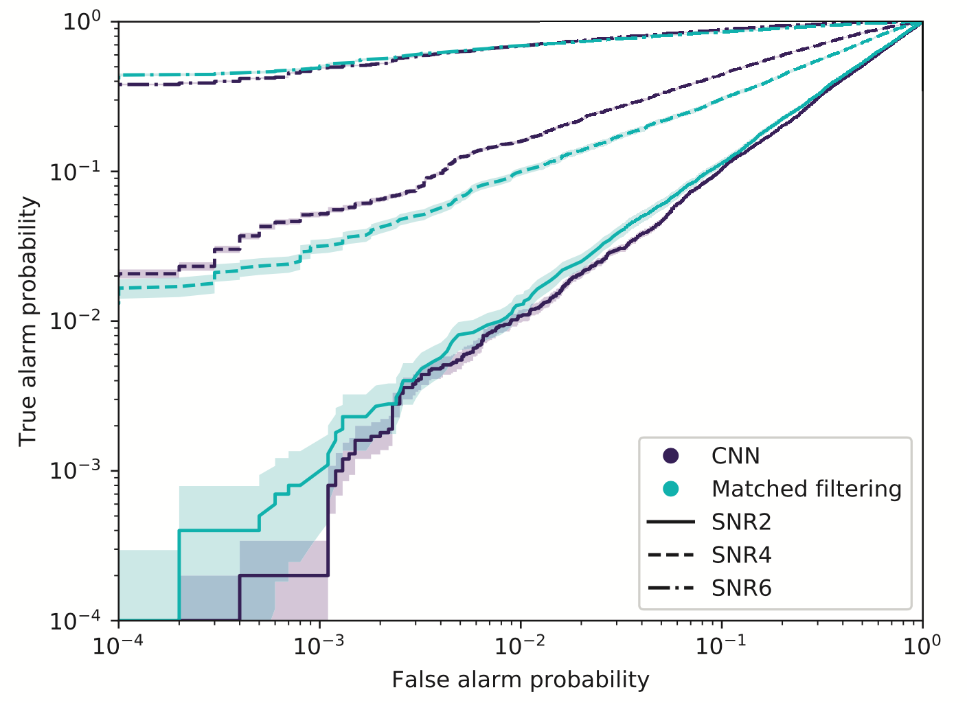
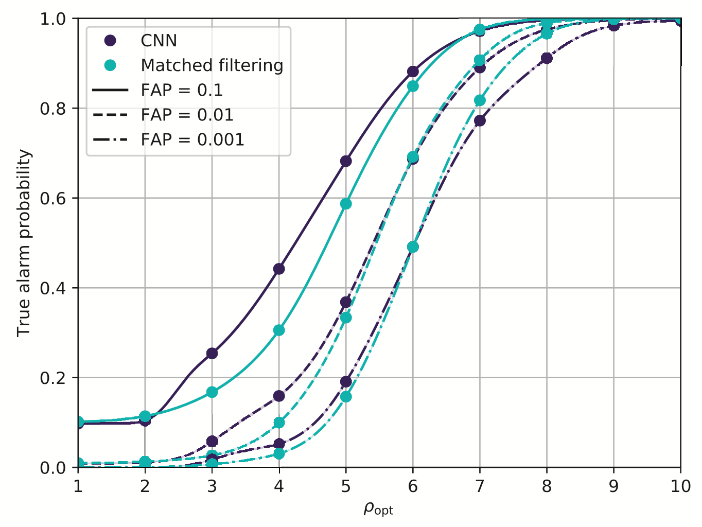
Proof-of-principle studies
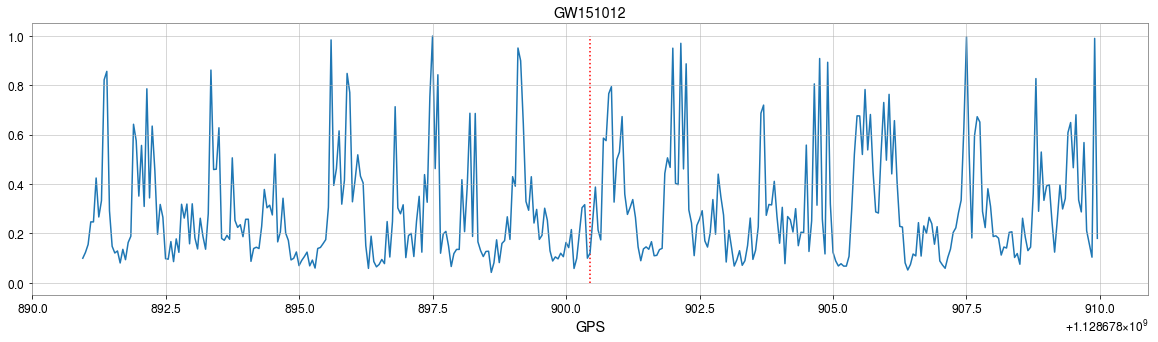
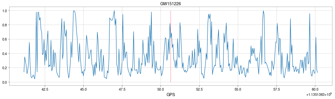
Production search studies
Milestones
More related works, see Survey4GWML (https://iphysresearch.github.io/Survey4GWML/)
Resilience to real non-Gaussian noise (Robustness)
Acceleration of existing pipelines (Speed, <0.1ms)
Stimulated background noises
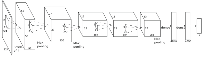
A specific design of the architecture is needed.
Classification
Feature extraction
Convolutional neural network (ConvNet or CNN)
A specific design of the architecture is needed.
Classification
Feature extraction
Convolutional neural network (ConvNet or CNN)
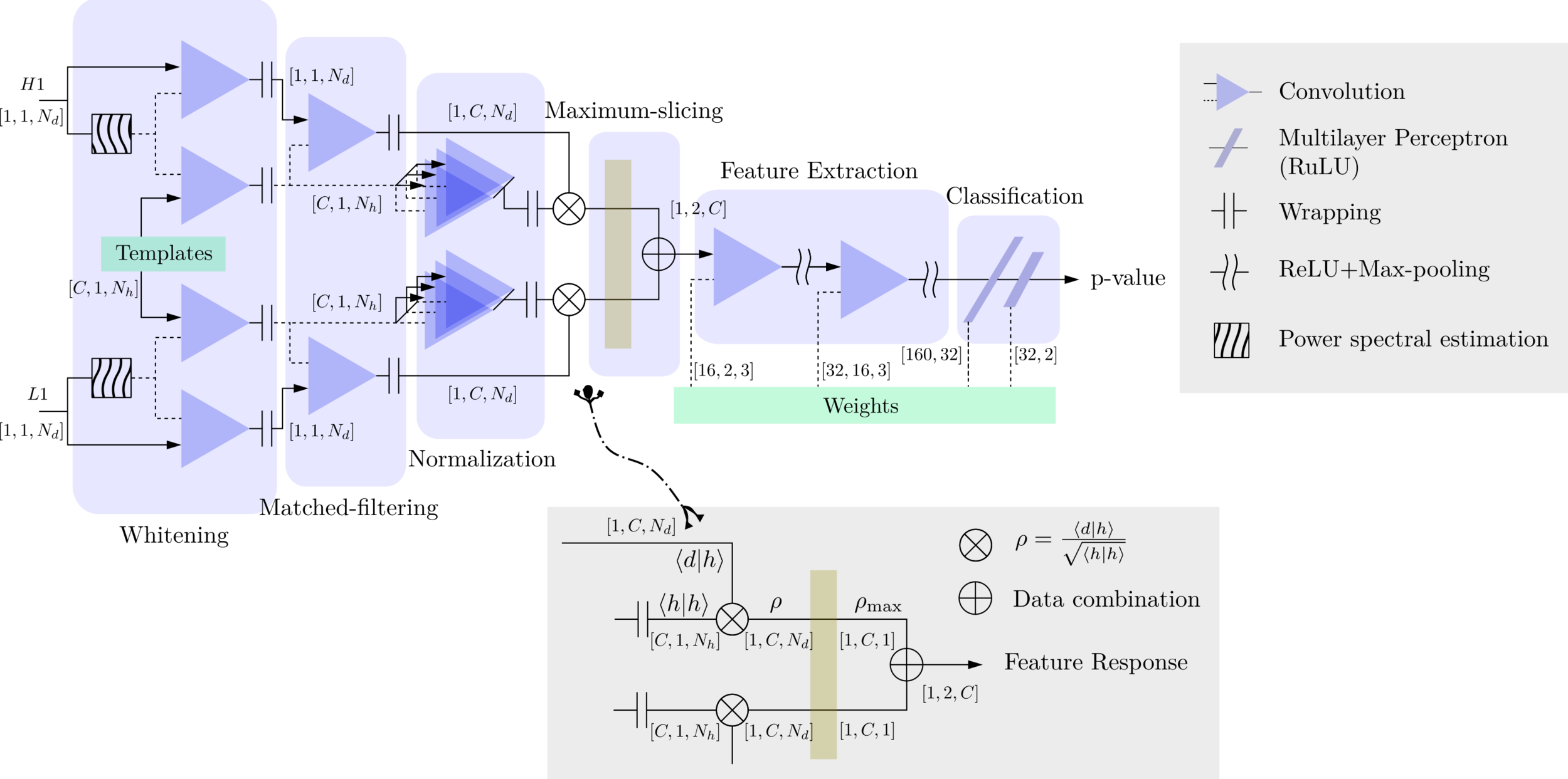
MFCNN
MFCNN
MFCNN
Classification
Feature extraction
Convolutional neural network (ConvNet or CNN)
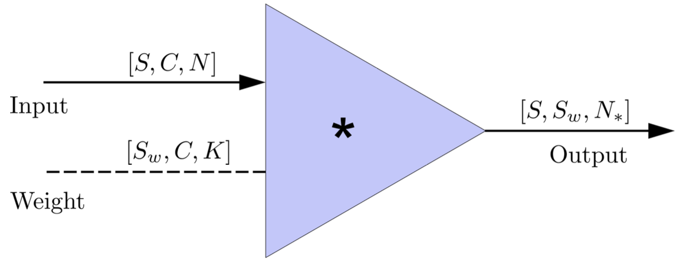
Matched-filtering (cross-correlation with the templates) can be regarded as a convolutional layer with a set of predefined kernels.
>> Is it matched-filtering ?
>> Wait, It can be matched-filtering!
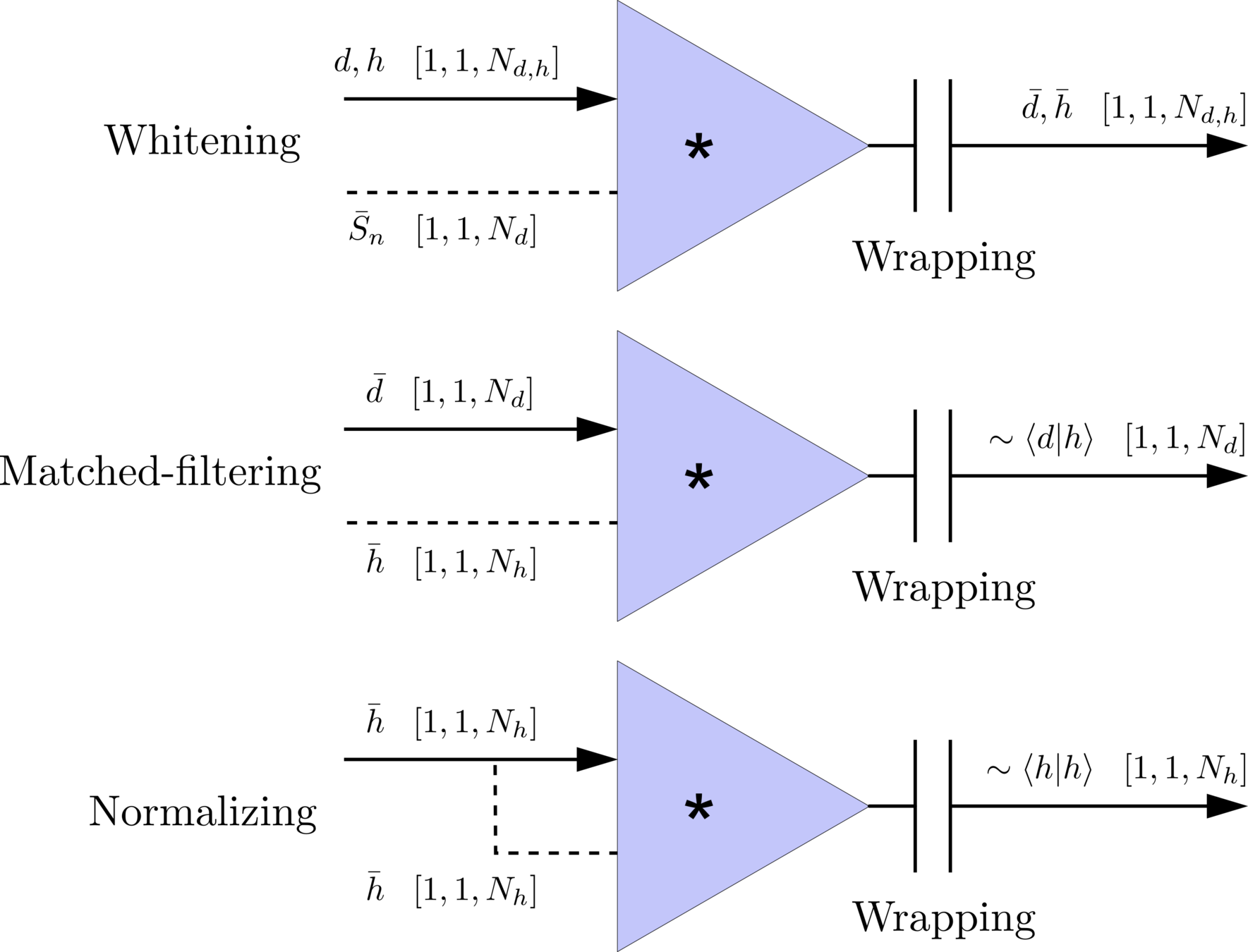
\(S_n(|f|)\) is the one-sided average PSD of \(d(t)\)
(whitening)
where
Time domain
Frequency domain
(normalizing)
(matched-filtering)
\(S_n(|f|)\) is the one-sided average PSD of \(d(t)\)
(whitening)
where
Time domain
Frequency domain
(normalizing)
(matched-filtering)
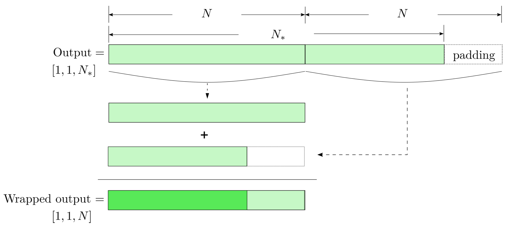
FYI: \(N_\ast = \lfloor(N-K+2P)/S\rfloor+1\)
(A schematic illustration for a unit of convolution layer)
\(S_n(|f|)\) is the one-sided average PSD of \(d(t)\)
(whitening)
where
Time domain
Frequency domain
(normalizing)
(matched-filtering)
Apache MXNet Framework
modulo-N circular convolution
Input
Output
Input
Output
Input
Output
import mxnet as mx
from mxnet import nd, gluon
from loguru import logger

def MFCNN(fs, T, C, ctx, template_block, margin, learning_rate=0.003):
    logger.success('Loading MFCNN network!')
    net = gluon.nn.Sequential()
    with net.name_scope():
        net.add(MatchedFilteringLayer(mod=fs*T, fs=fs,
                                      template_H1=template_block[:,:1],
                                      template_L1=template_block[:,-1:]))
        net.add(CutHybridLayer(margin = margin))
        net.add(Conv2D(channels=16, kernel_size=(1, 3), activation='relu'))
        net.add(MaxPool2D(pool_size=(1, 4), strides=2))
        net.add(Conv2D(channels=32, kernel_size=(1, 3), activation='relu'))
        net.add(MaxPool2D(pool_size=(1, 4), strides=2))
        net.add(Flatten())
        net.add(Dense(32))
        net.add(Activation('relu'))
        net.add(Dense(2))
	# Initialize parameters of all layers
    net.initialize(mx.init.Xavier(magnitude=2.24), ctx=ctx, force_reinit=True)
    return net
The available codes: https://gist.github.com/iphysresearch/a00009c1eede565090dbd29b18ae982c
input
GW Data from GWOSC: https://www.gw-openscience.org/
This slide: https://slides.com/iphysresearch/apachemxnet_mfcnn
input
for _ in range(num_of_audiences):
    print('Thank you for your attention!')
Profile: iphysresearch.github.io/-he.wang/
Twitter: twitter.com/@Herb_hewang
GW Data from GWOSC: https://www.gw-openscience.org/
This slide: https://slides.com/iphysresearch/apachemxnet_mfcnn
By He Wang
Apache MXNet Day, 10:01 AM PST on December 14th, 2020


