Gravitational-wave Signal Recognition of LIGO Data by Deep Learning



He Wang (王赫)
Institute of Theoretical Physics, CAS
Beijing Normal University
on behalf of the KAGRA collaboration
中国物理学会引力与相对论天体物理分会 , 14:40-15:00 on April 24\(^\text{th}\), 2021
Based on DOI: 10.1103/physrevd.101.104003,

hewang@mail.bnu.edu.cn / hewang@itp.ac.cn
Content
- Introduction
- Challenge & Opportunity
- Attempts on stimulated/real data
- Matched-filtering Convolutional Neural Network (MFCNN)
- Configuration & Search Strategy
- Results: GW events in GWTC-1 & GWTC-2
- Trends & Outlook
Gravitational-wave Astronomy
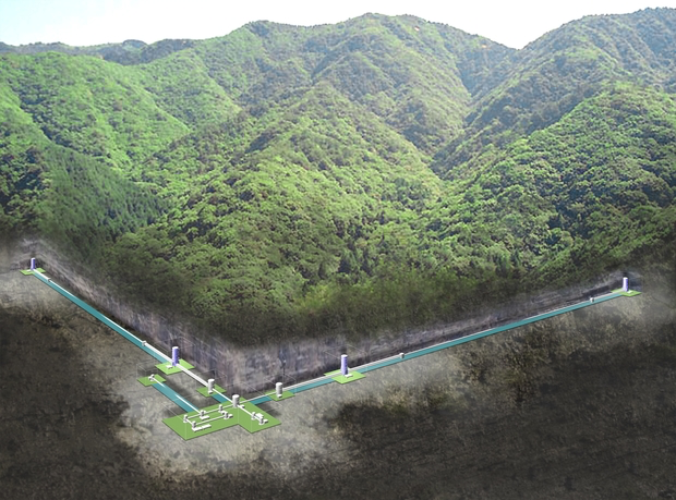
- Advanced LIGO observing since 2015 (two detectors in US), joined by Virgo (Italy) in 2017 and KAGRA (Japan) in Japan in 2020.
- Best GW hunter in the range 10Hz-10kHz.


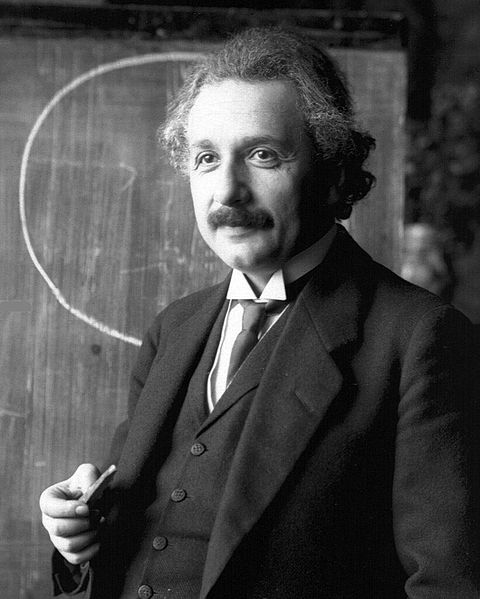
- 100 years from Einstein's prediction to the first LIGO-Virgo detection (GW150914) announcement in 2016.
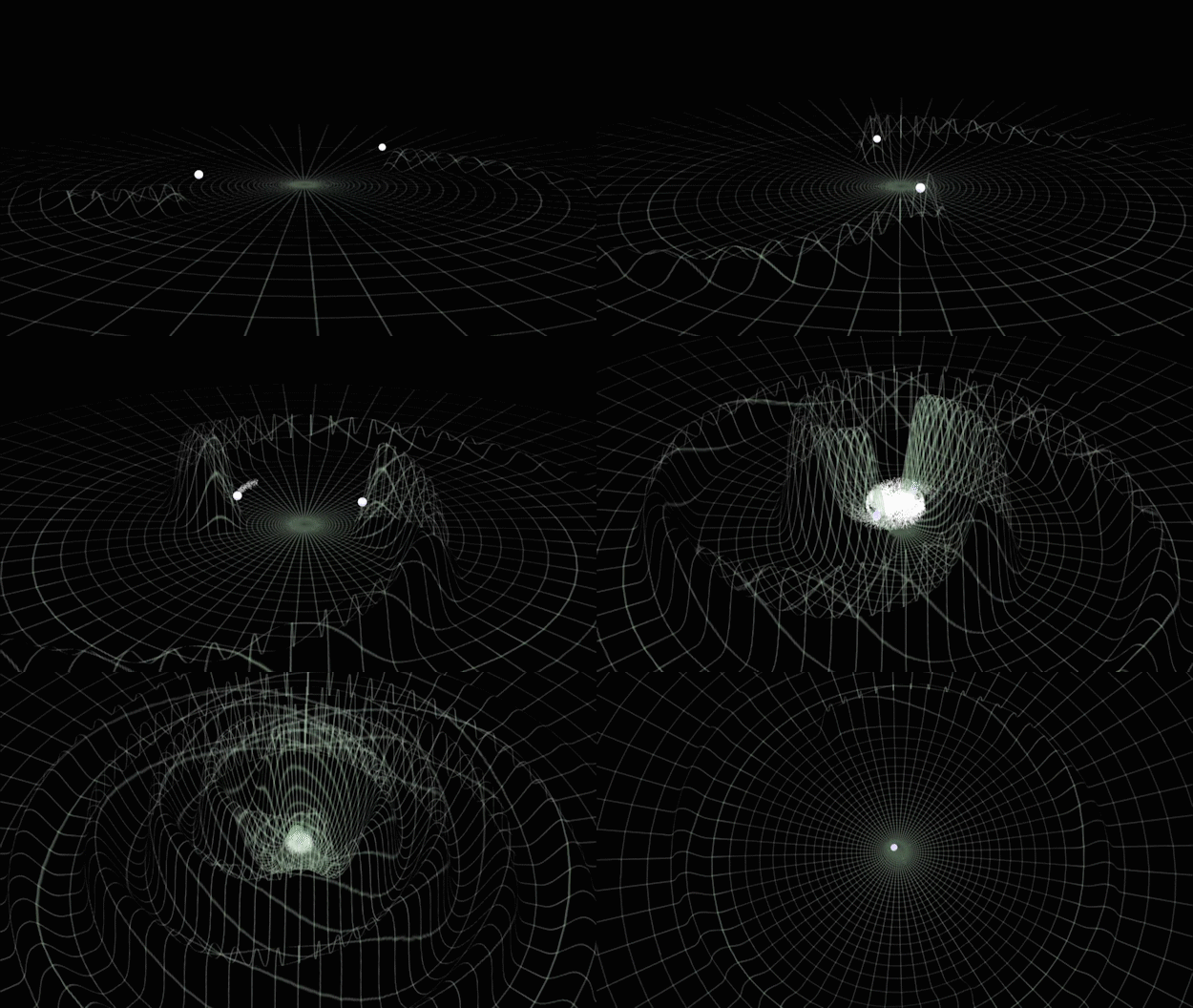
- General relativity: "Spacetime tells matter how to move, and matter tells spacetime how to curve."
- Time-varying quadrupolar mass distributions lead to propagating ripples in spacetime: GWs.
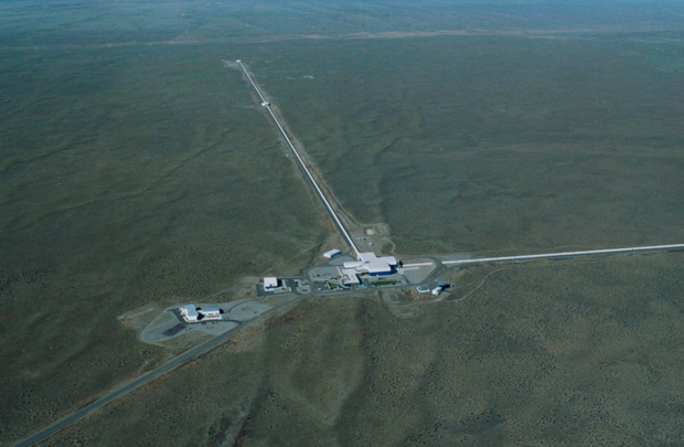
LIGO Hanford (H1)
KAGRA
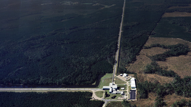
LIGO Livingston (L1)
Noise power spectral density (one-sided)
-
Matched-filtering Technique (prior-free Neyman-Pearson Framework):
- It is an optimal linear filter for weak signals buried in the Gaussian and stationary noise \(n(t)\).
- Works by correlating a known signal model \(h(t)\) (template) with the data.
- Starting with data: \(d(t) = h(t) + n(t)\).
- Defining the matched-filtering SNR \(\rho(t)\):
where
- The 4-D search parameter space in the first observation run covered by a template bank to circular binaries for which the spin of the systems is aligned (or antialigned) with the orbital angular momentum of the binary.
- ~250,000 template waveforms are used for O1 (computationally expansive).
The template that best matches GW150914 event
Challenges in GW Data Analysis
Opportunities in GW Data Analysis
-
Phys.Rev.D 97 (2018) 4, 044039
- The first attempt
-
Phys.Rev.Lett 120 (2019) 14, 141103
- Matched-filtering vs CNN
-
Phys.Rev.D 101, 083006 (2020)
- GstLAL vs DNN by ranking candidates...
-
Phys.Rev.D 100 (2019) 6, 063015
- GW events for BBH in GWTC-1
-
Phys.Rev.D 101 (2020) 10, 104003
- All GW events in GWTC-1
-
Phys.Rev.D 103 (2021), 063034
- Periods of 7 BBH events in O2
-
Phys.Lett.B 812 (2021) 136029
- GWTC-1 & GW190412, GW190521
-
2011.10425
- GWTC-1 & 34/37 in GWTC-2
Proof-of-principle studies
Production search studies
Milestones
More related works, see 2005.03745 or Survey4GWML (https://iphysresearch.github.io/Survey4GWML/)
- When machine & deep learning meets GW astronomy:
- Covering more parameter-space (Interpolation)
- Automatic generalization to new sources (Extrapolation)
-
Resilience to real non-Gaussian noise (Robustness)
-
Acceleration of existing pipelines (Speed, <0.1ms)
-
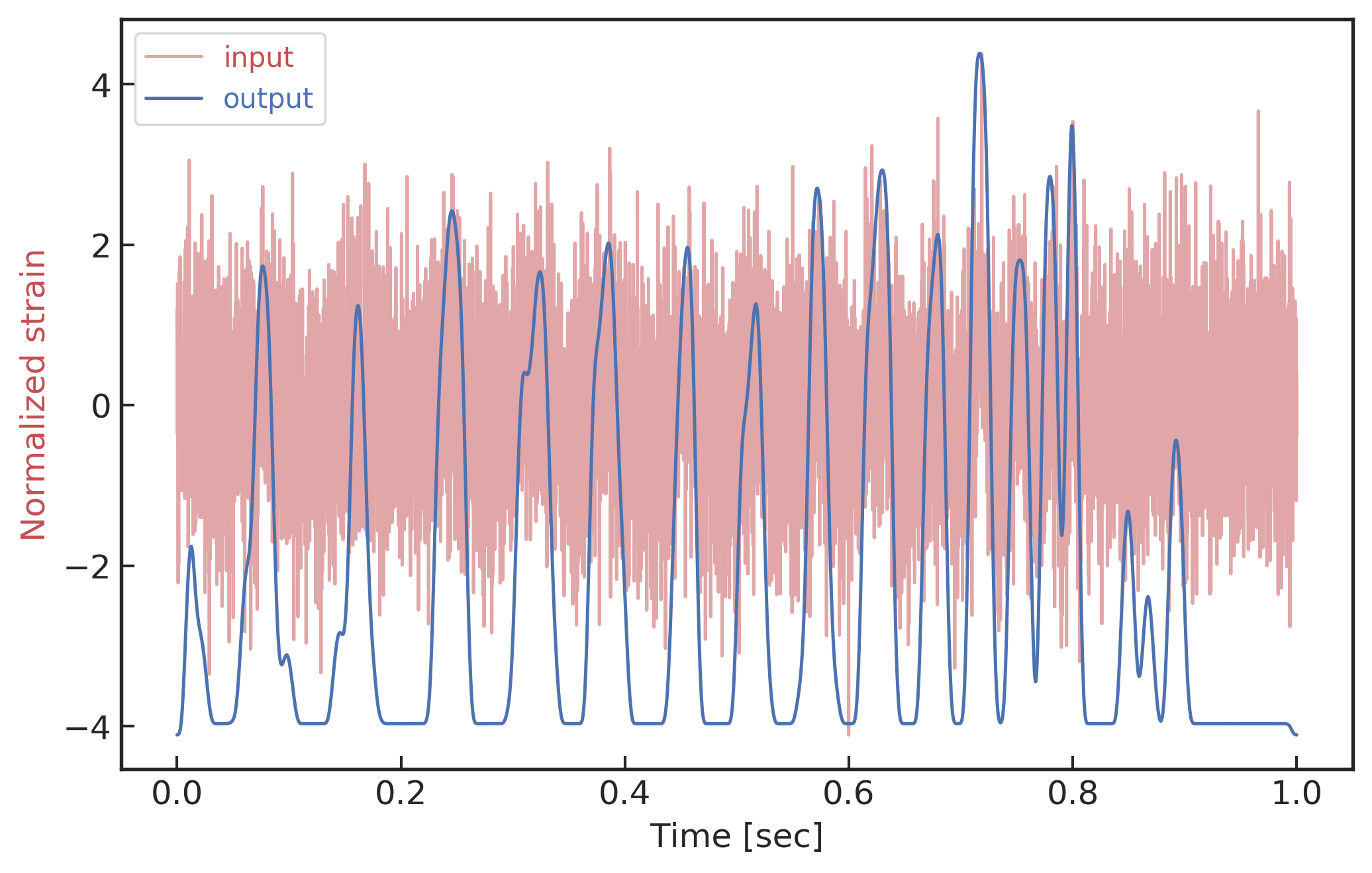
Task: Whether or not a given noisy data contain a GW signal? (classification problem)
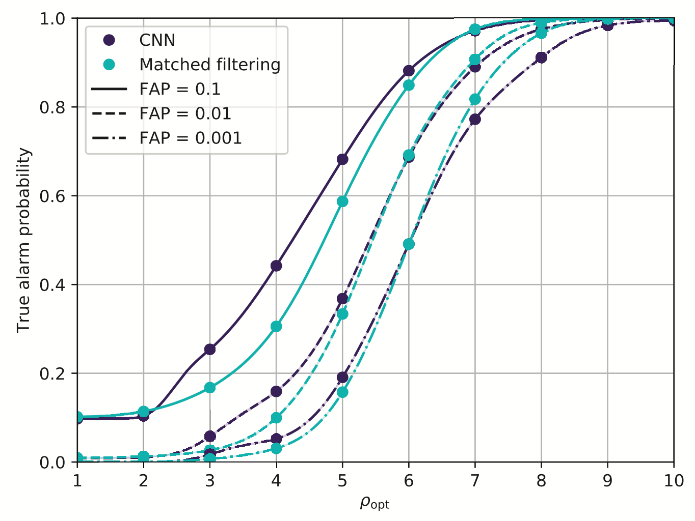
Stimulated background noises
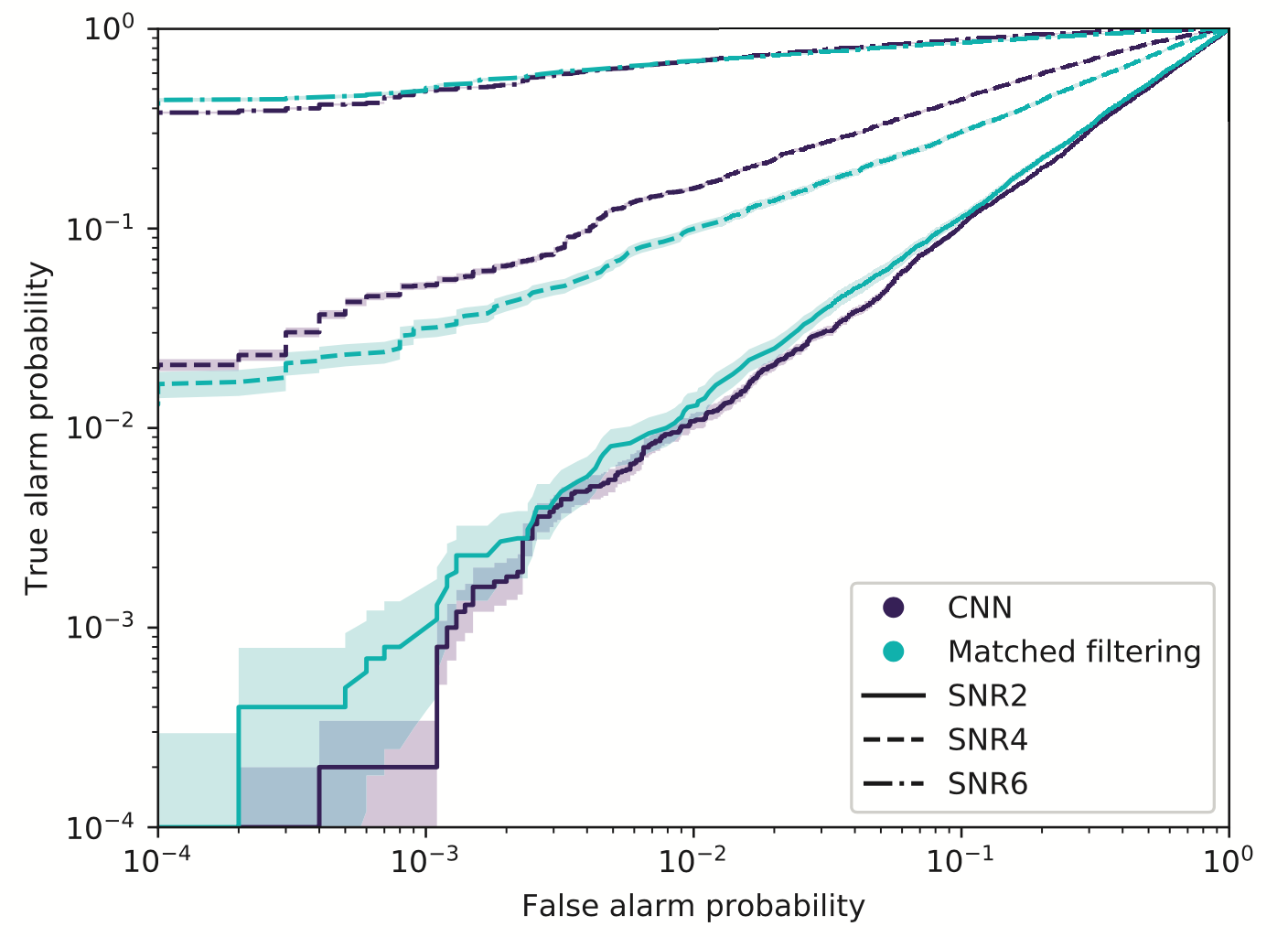
- CNNs structure performs as well as the standard matched filter method in extracting BBH signals under non-ideal conditions.
Last updated on Nov. 2020
Past attempts on stimulated noise
Classification

Feature extraction
Convolutional Neural Network (ConvNet or CNN)
- Fine-tune the Convolutional Neural Network
- A glimpse of model interpretability using data visualization.
- Identify what kind of feature is learned.
\(\rightarrow\) Deeper means better. But no more than ~3 layer. Marginal!
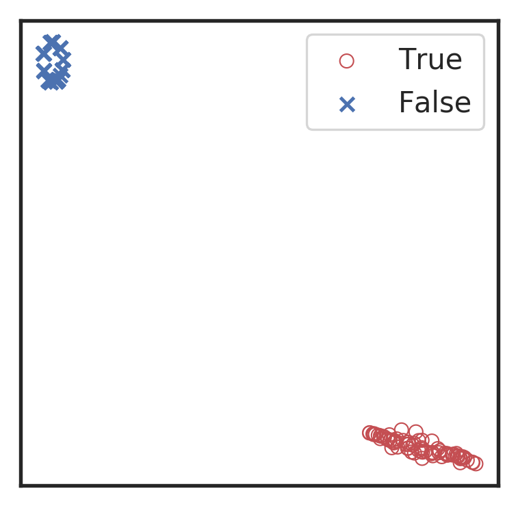
Visualization for the high-dimensional feature maps of learned network in layers for bi-class using t-SNE.
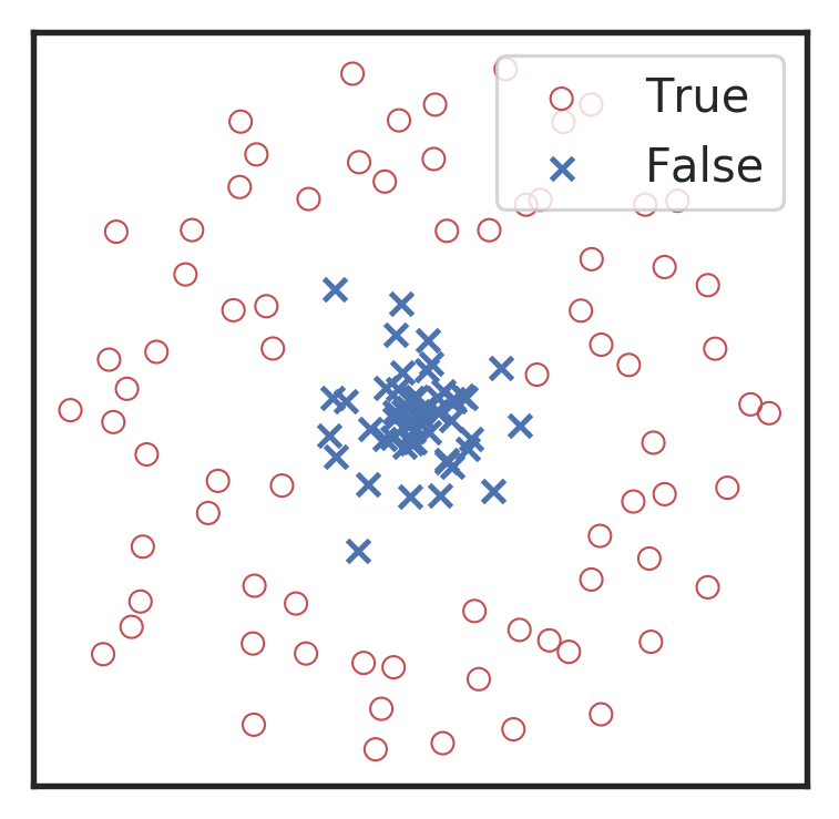
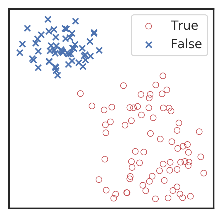
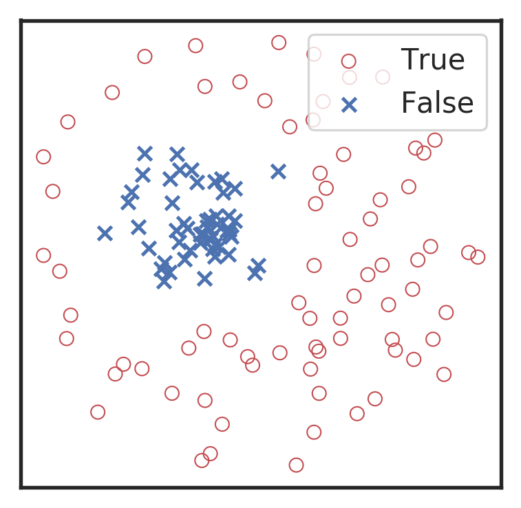
Related works:
the 1st layer
the 2nd layer
the 3rd layer
the last layer
\(\rightarrow\)High sensitivity on the merge part of GW waveform
\(\rightarrow\)Extracted features play a decisive role.

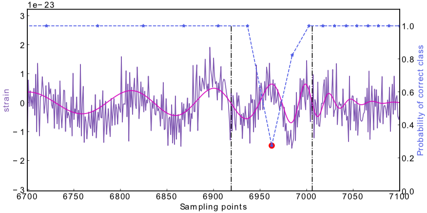
Occlusion Sensitivity
Attempts on Real LIGO Noise


- CNNs always works pretty good on stimulated noises.
- However, when on real noises from LIGO, this approach does not work that well.
- It's too sensitive against the background + hard to find GW events)
A specific design of the architecture is needed.
GW150914
GW151226
GW151012
Classification

Feature extraction
Convolutional Neural Network (ConvNet or CNN)


MFCNN
MFCNN
MFCNN
Result on Real LIGO Noise
- CNNs always works pretty good on stimulated noises.
- However, when on real noises from LIGO, this approach does not work that well.
- It's too sensitive against the background + hard to find GW events)
Classification

Feature extraction
Convolutional Neural Network (ConvNet or CNN)
A specific design of the architecture is needed.
GW150914
GW151226
GW151012
Motivation
- With the closely related concepts between the templates and kernels , we attempt to address a question of:
Matched-filtering (cross-correlation with the templates) can be regarded as a convolutional layer with a set of predefined kernels.
>> Is it matched-filtering ?
>> Wait, It can be matched-filtering!
- In practice, we use matched filters as an essential component of feature extraction in the first part of the CNN for GW detection.
Classification

Feature extraction
Convolutional Neural Network (ConvNet or CNN)
\(S_n(|f|)\) is the one-sided average PSD of \(d(t)\)
(whitening)
where
Time domain
Frequency domain
(normalizing)
(matched-filtering)
Deep Learning Framework
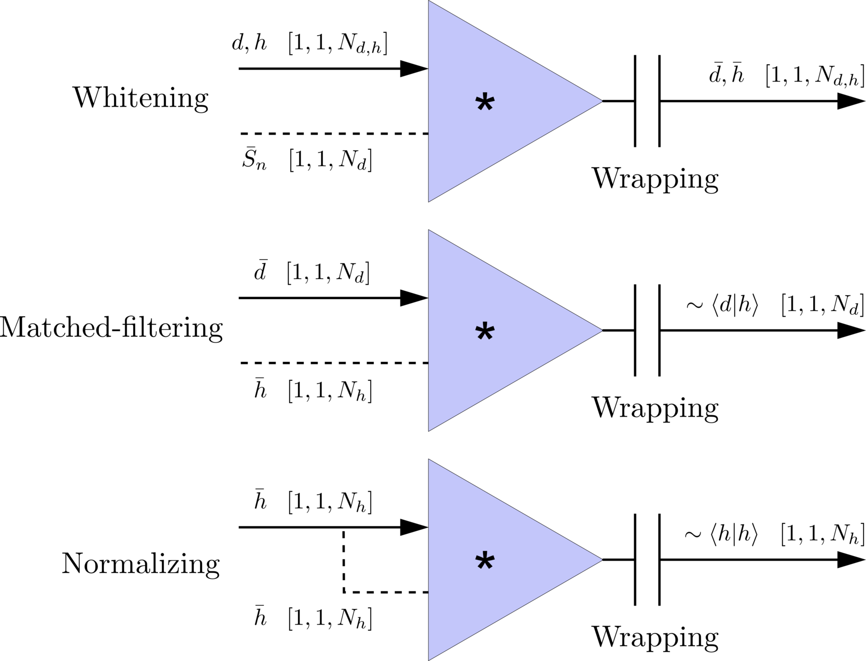


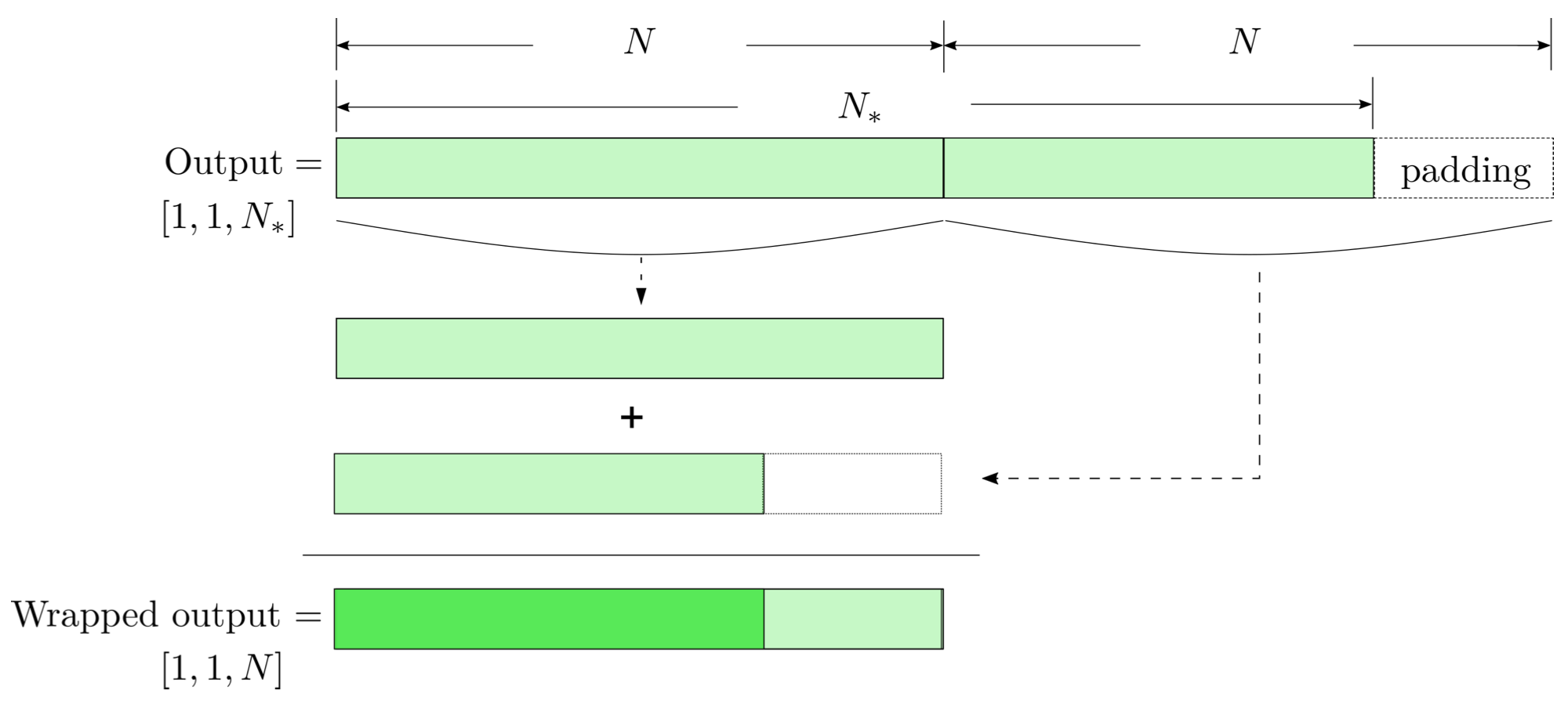
modulo-N circular convolution
Matched-filtering CNNs (MFCNN)
- Transform matched-filtering method from frequency domain to time domain.
- The square of matched-filtering SNR for a given data \(d(t) = n(t)+h(t)\):
\(S_n(|f|)\) is the one-sided average PSD of \(d(t)\)
(whitening)
where
Time domain
Frequency domain
(normalizing)
(matched-filtering)
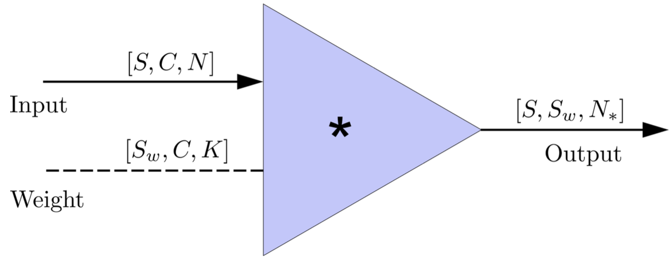
- In the 1-D convolution (\(*\)) on Apache MXNet, given input data with shape [batch size, channel, length] :
FYI: \(N_\ast = \lfloor(N-K+2P)/S\rfloor+1\)
(A schematic illustration for a unit of convolution layer)
Deep Learning Framework
Matched-filtering CNNs (MFCNN)
- Transform matched-filtering method from frequency domain to time domain.
- The square of matched-filtering SNR for a given data \(d(t) = n(t)+h(t)\):
- The structure of MFCNN:
Input
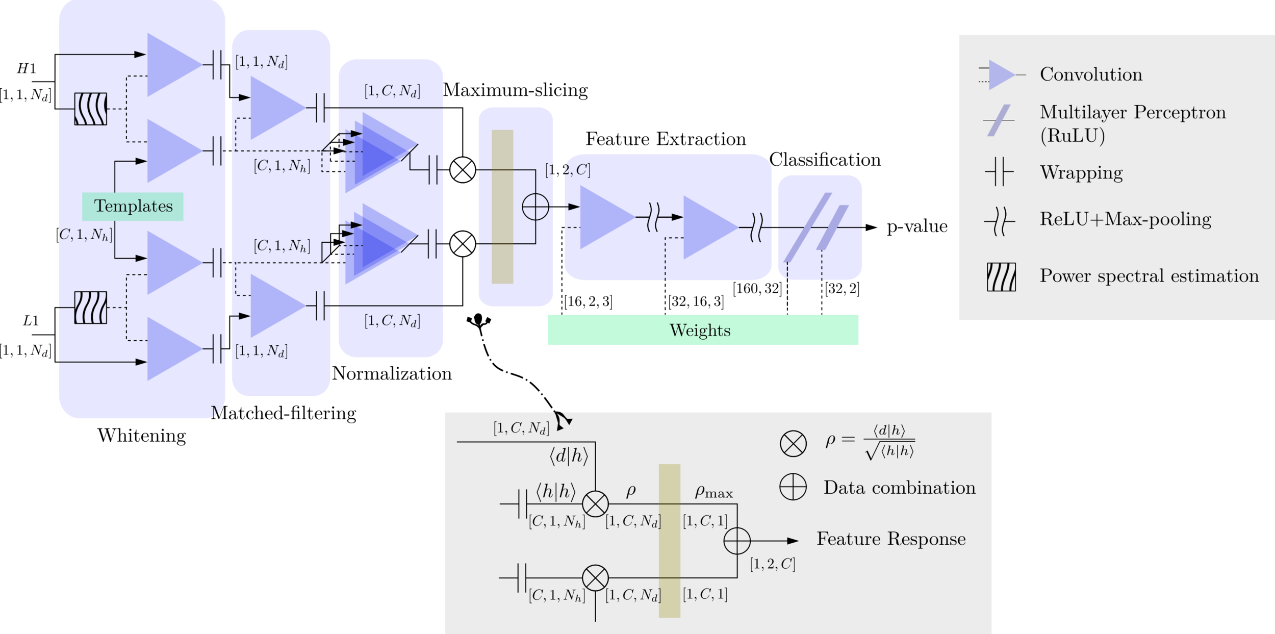

Output
- In the meanwhile, we can obtain the optimal time \(N_0\) (relative to the input) of feature response of matching by recording the location of the maxima value corresponding to the optimal template \(C_0\).
Matched-filtering CNNs (MFCNN)
Input


Output
- In the meanwhile, we can obtain the optimal time \(N_0\) (relative to the input) of feature response of matching by recording the location of the maxima value corresponding to the optimal template \(C_0\).
import mxnet as mx
from mxnet import nd, gluon
from loguru import logger

def MFCNN(fs, T, C, ctx, template_block, margin, learning_rate=0.003):
    logger.success('Loading MFCNN network!')
    net = gluon.nn.Sequential()
    with net.name_scope():
        net.add(MatchedFilteringLayer(mod=fs*T, fs=fs,
                                      template_H1=template_block[:,:1],
                                      template_L1=template_block[:,-1:]))
        net.add(CutHybridLayer(margin = margin))
        net.add(Conv2D(channels=16, kernel_size=(1, 3), activation='relu'))
        net.add(MaxPool2D(pool_size=(1, 4), strides=2))
        net.add(Conv2D(channels=32, kernel_size=(1, 3), activation='relu'))
        net.add(MaxPool2D(pool_size=(1, 4), strides=2))
        net.add(Flatten())
        net.add(Dense(32))
        net.add(Activation('relu'))
        net.add(Dense(2))
	# Initialize parameters of all layers
    net.initialize(mx.init.Xavier(magnitude=2.24), ctx=ctx, force_reinit=True)
    return net
The available codes: https://gist.github.com/iphysresearch/a00009c1eede565090dbd29b18ae982c
1 sec duration
35 templates used

- The structure of MFCNN:
Matched-filtering CNNs (MFCNN)
Training Configuration and Search Methodology
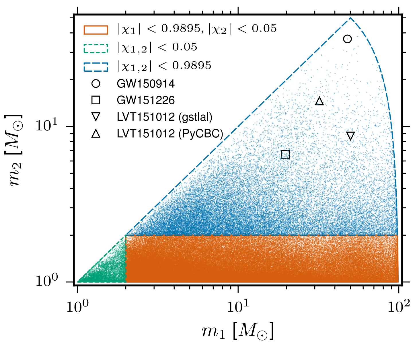
- We use SEOBNRE model [Cao et al. (2017), Liu et al. (2020)] to generate waveform, we only consider circular, spinless binary black holes.
- The background noises for training/testing are sampled from a small closed set (33*4096s) in the first observation run (O1) in the absence of the segments (4096s) containing the first 3 GW events.
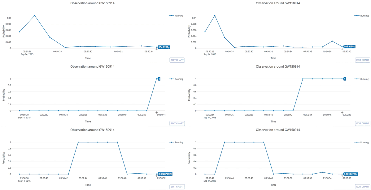
- Every 5 seconds segment as input of our MF-CNN with a step size of 1 second.
- The model can scan the whole range of the input segment and output a probability score.
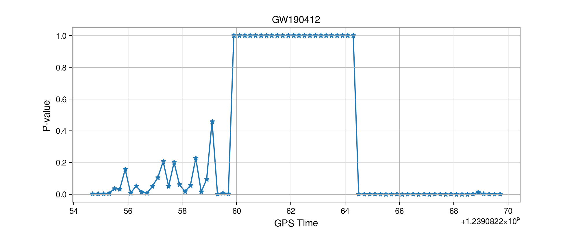
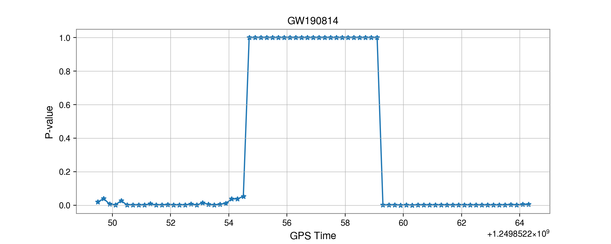
- In the ideal case, with a GW signal hiding in somewhere, there should be 5 adjacent predictions for it with respect to a threshold.
FYI: sampling rate = 4096Hz
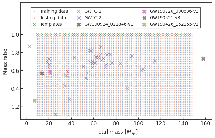
| templates | waveforms (train/test) | |
|---|---|---|
| Number | 35 | 1610 |
| Length (sec) | 1 | 5 |
| equal mass |
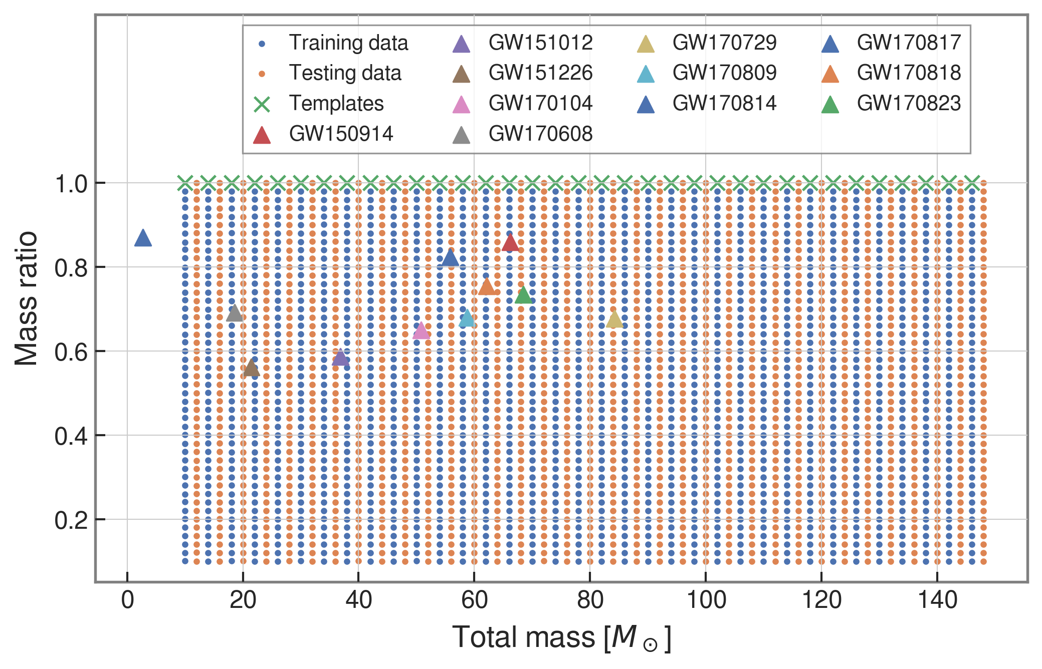


input
- Recovering the three GW events in O1.
- Recovering all GW events in O2, even including GW170817 event.


Results: GW events in GWTC-1


- Recovering the three GW events in O1.
- Recovering all GW events in O2, even including GW170817 event.
Results: GW events in GWTC-1
- Recovering the three GW events in O1.
- Recovering all GW events in O2, even including GW170817 event.
- (Some results on statistical significance on O1 data & glitches identification have skipped here)
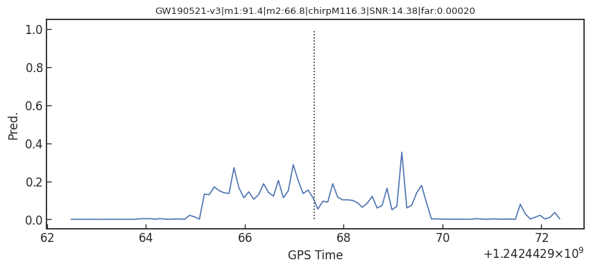
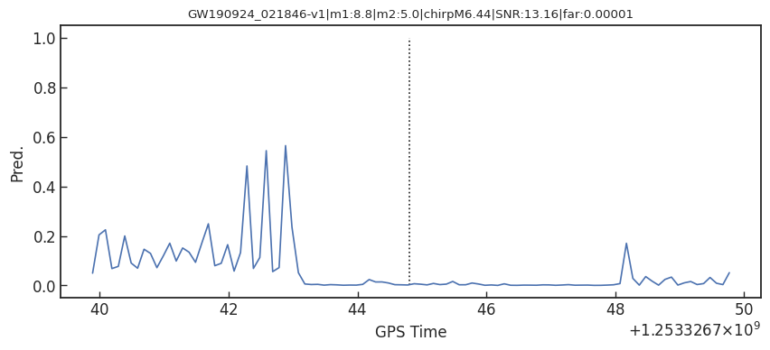
- Consider 33 events (with H1 detector data) in O3a (39 events in total), 4 of them are misclassified.
GW170817
GW190814
GW190412
- Selected events:


Results: GW events in GWTC-1 & GWTC-2

GW170817
GW190814
GW190412


Summary & Lesson Learned
- Some benefits from MFCNN architecture for GW detection:
- Recovering all GW events in GWTC-1 and 29 of 33 GW events in GWTC-2 (39 events in total).
- We realized that:
- GW templates can be used as likely known features for signal recognition.
- Generalization of both matched-filtering and neural networks.
- Linear filters (i.e. matched-filtering) in signal processing can be rewritten as neural layers (i.e. CNNs).
- Recovering the three GW events in O1.
- Recovering all GW events in O2, even including GW170817 event.
- (Some results on statistical significance on O1 data & glitches identification have skipped here)
- Consider 33 events (with H1 detector data) in O3a (39 events in total), 4 of them are misclassified.
- Selected events:
Results: GW events in GWTC-1 & GWTC-2


Trends & Outlook
-
Phys.Rev.D 97 (2018) 4, 044039
- The first attempt
-
Phys.Rev.Lett 120 (2019) 14, 141103
- Matched-filtering vs CNN
-
Phys.Rev.D 101, 083006 (2020)
- GstLAL vs DNN by ranking candidates...
-
Phys.Rev.D 100 (2019) 6, 063015
- GW events for BBH in GWTC-1
-
Phys.Rev.D 101 (2020) 10, 104003
- All GW events in GWTC-1
-
Phys.Lett.B 812 (2021) 136029
- GWTC-1 & GW190412, GW190521
-
2011.10425
- GWTC-1 & 34/37 in GWTC-2
-
Phys.Rev.D 103, 062004 (2021)
- 8/11 in GWTC-1
-
Phys.Lett.B 815 (2021) 136161
- All GW events in GWTC-1
Proof-of-principle studies
Production search studies
Current paradigm:
- Change your input data: Time series vs time-frequency domain
- Pre-feature-extraction to lower the bar
- MFCNN、Wavelet decomposition (Front.Phys. 15, 54501 (2020))
- Use more powerful model (“Give Me”): ResNet/Wavenet/LSTM...
More related works, see 2005.03745 or Survey4GWML (https://iphysresearch.github.io/Survey4GWML/)
Last updated on April. 2021
Drawbacks:
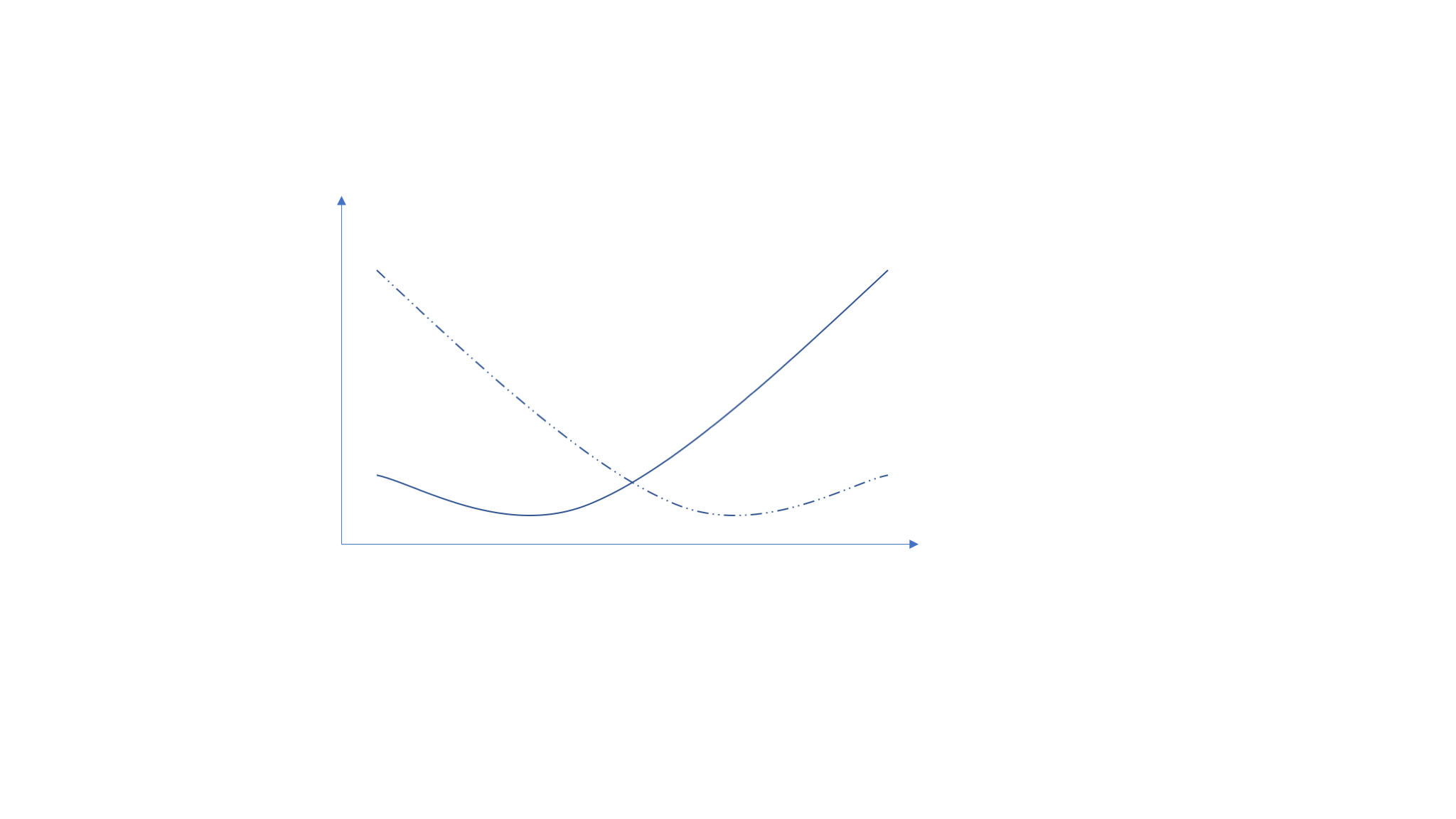
- The output of neural network (Softmax function) is not an optimal and reasonable detection statistic.
- "The negative log-likelihood cost function always strongly penalizes the most active incorrect prediction. And the correctly classified examples will contribute little to the overall training cost."
—— I. Goodfellow, Y. Bengio, A. Courville. Deep Learning.
Softmax function

Score
Pred.
Noise
Noise + Signal
Pred.
Possible ways to resolve the problem:
- Bridge the gap between ML and MF (MFCNN, 2104.03961)
- Fast posterior density estimation with ML (in preparation)
- ...
Detection of early inspiral of GW
- Phys.Rev.D 103 (2021), 063034
- Wei et al. (2012.03963)
- Baltus et al. (2104.00594)
- Yu et al. (2104.09438)

for _ in range(num_of_audiences):
    print('Thank you for your attention! 🙏')
This slide: https://slides.com/iphysresearch/gra2020-2021
Trends & Outlook
-
Phys.Rev.D 97 (2018) 4, 044039
- The first attempt
-
Phys.Rev.Lett 120 (2019) 14, 141103
- Matched-filtering vs CNN
-
Phys.Rev.D 101, 083006 (2020)
- GstLAL vs DNN by ranking candidates...
-
Phys.Rev.D 100 (2019) 6, 063015
- GW events for BBH in GWTC-1
-
Phys.Rev.D 101 (2020) 10, 104003
- All GW events in GWTC-1
-
Phys.Lett.B 812 (2021) 136029
- GWTC-1 & GW190412, GW190521
-
2011.10425
- GWTC-1 & 34/37 in GWTC-2
-
Phys.Rev.D 103, 062004 (2021)
- 8/11 in GWTC-1
-
Phys.Lett.B 815 (2021) 136161
- All GW events in GWTC-1
Proof-of-principle studies
Production search studies
Current paradigm:
- Change your input data: Time series vs time-frequency domain
- Pre-feature-extraction to lower the bar
- MFCNN、Wavelet decomposition (Front.Phys. 15, 54501 (2020))
- Use more powerful model (“Give Me”): ResNet/Wavenet/LSTM...
More related works, see 2005.03745 or Survey4GWML (https://iphysresearch.github.io/Survey4GWML/)
Last updated on April. 2021
Drawbacks:
- The output of neural network (Softmax function) is not an optimal and reasonable detection statistic.
- "The negative log-likelihood cost function always strongly penalizes the most active incorrect prediction. And the correctly classified examples will contribute little to the overall training cost."
—— I. Goodfellow, Y. Bengio, A. Courville. Deep Learning.
Softmax function

Score
Pred.

Noise
Noise + Signal
Pred.
Possible ways to resolve the problem:
- Bridge the gap between ML and MF (MFCNN, 2104.03961)
- Fast posterior density estimation with ML (in preparation)
- ...
Detection of early inspiral of GW
- Phys.Rev.D 103 (2021), 063034
- Wei et al. (2012.03963)
- Baltus et al. (2104.00594)
- Yu et al. (2104.09438)
