


He Wang PRO
Knowledge increases by sharing but not by saving.
He Wang (王赫)
Institute of Theoretical Physics, CAS
Beijing Normal University
on behalf of the KAGRA collaboration
中国物理学会引力与相对论天体物理分会 , 14:40-15:00 on April 24\(^\text{th}\), 2021
Based on DOI: 10.1103/physrevd.101.104003,
hewang@mail.bnu.edu.cn / hewang@itp.ac.cn
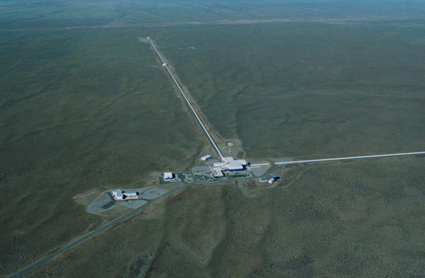
LIGO Hanford (H1)
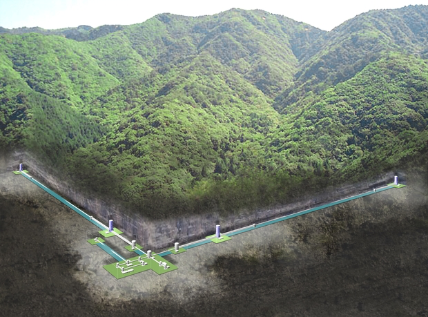
KAGRA
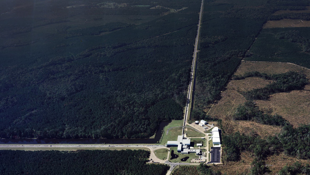
LIGO Livingston (L1)
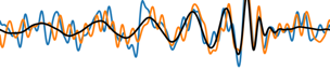
Noise power spectral density (one-sided)
where
The template that best matches GW150914 event
Proof-of-principle studies
Production search studies
Milestones
More related works, see 2005.03745 or Survey4GWML (https://iphysresearch.github.io/Survey4GWML/)
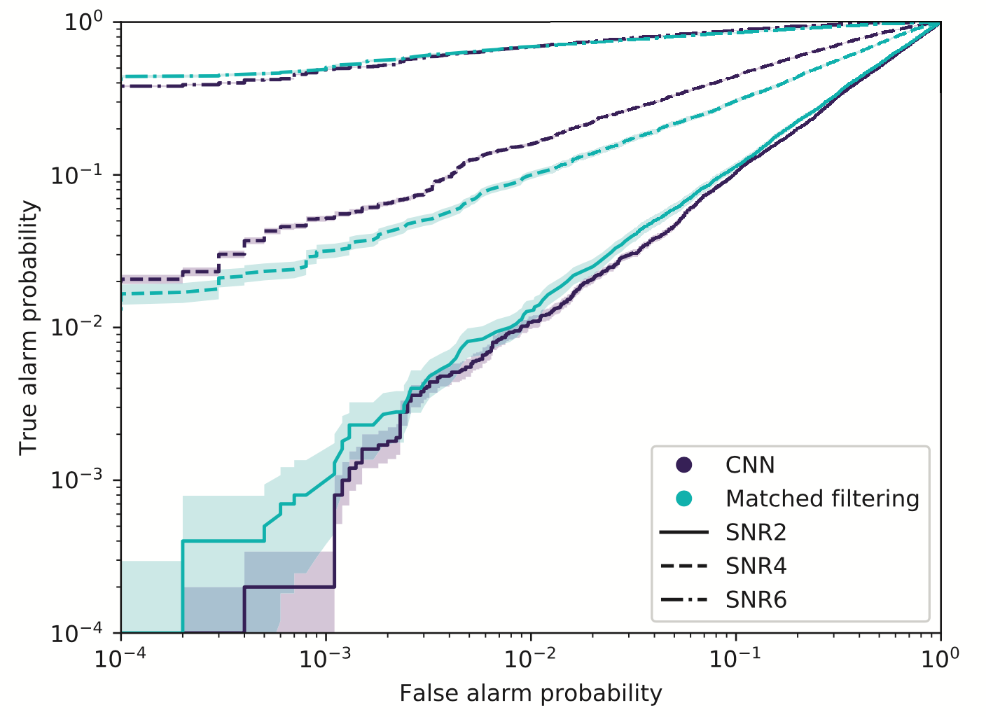
Resilience to real non-Gaussian noise (Robustness)
Acceleration of existing pipelines (Speed, <0.1ms)
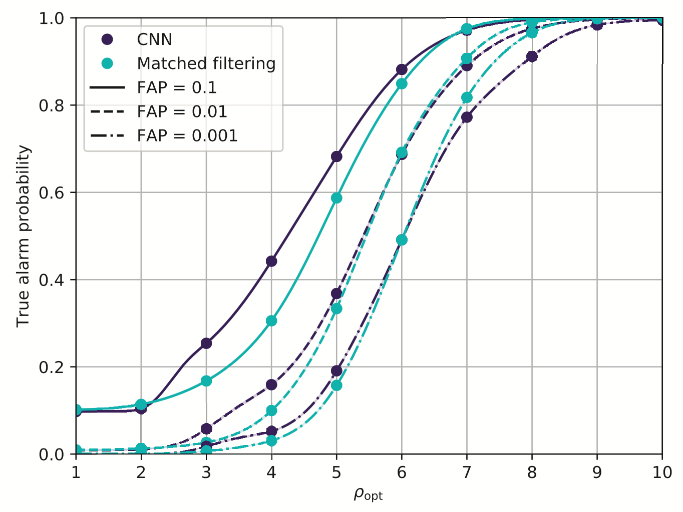
Task: Whether or not a given noisy data contain a GW signal? (classification problem)
Stimulated background noises
Last updated on Nov. 2020
Classification
Feature extraction
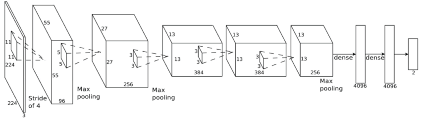
Convolutional Neural Network (ConvNet or CNN)
\(\rightarrow\) Deeper means better. But no more than ~3 layer. Marginal!
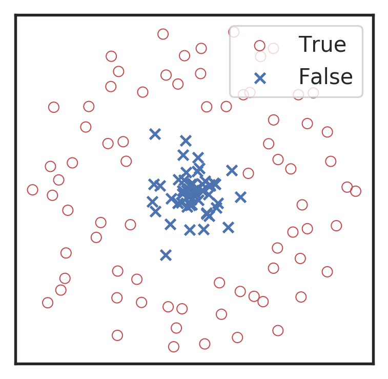
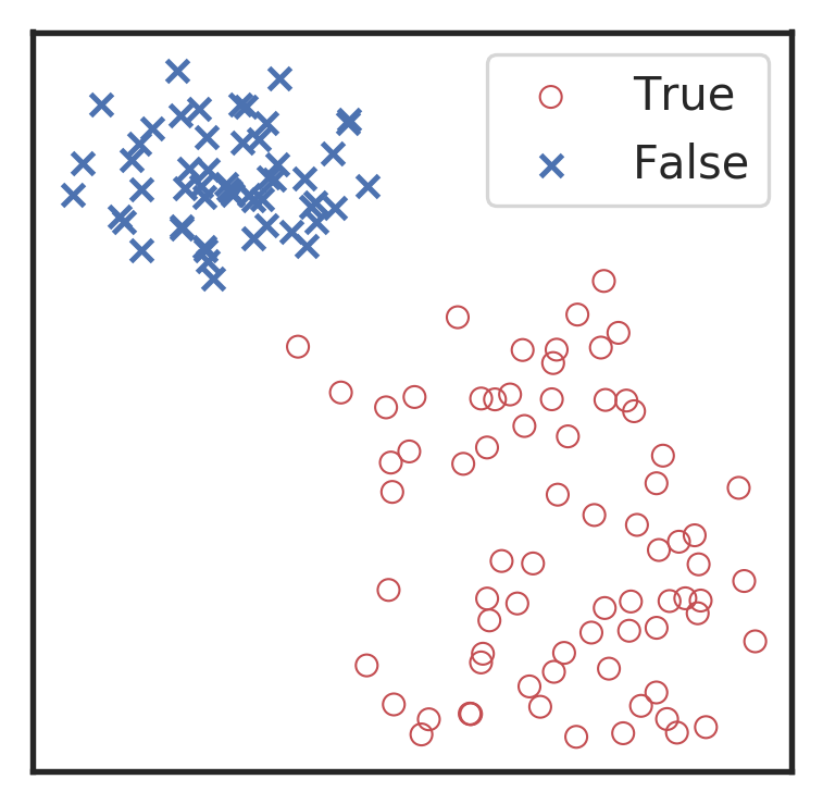
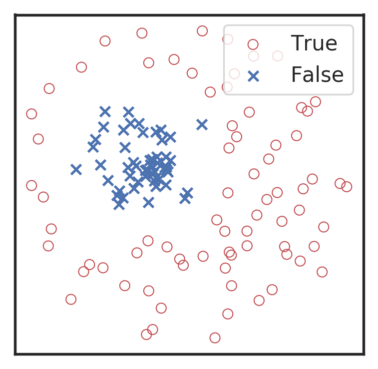
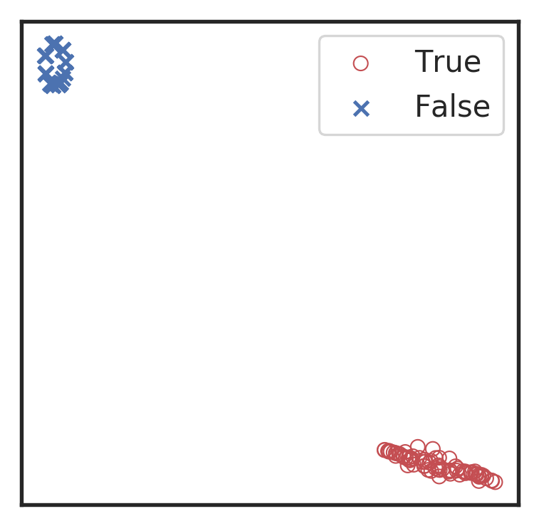
Visualization for the high-dimensional feature maps of learned network in layers for bi-class using t-SNE.
Related works:
the 1st layer
the 2nd layer
the 3rd layer
the last layer
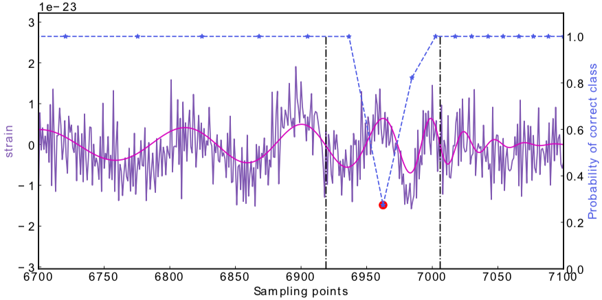
\(\rightarrow\)High sensitivity on the merge part of GW waveform
\(\rightarrow\)Extracted features play a decisive role.
Occlusion Sensitivity
A specific design of the architecture is needed.
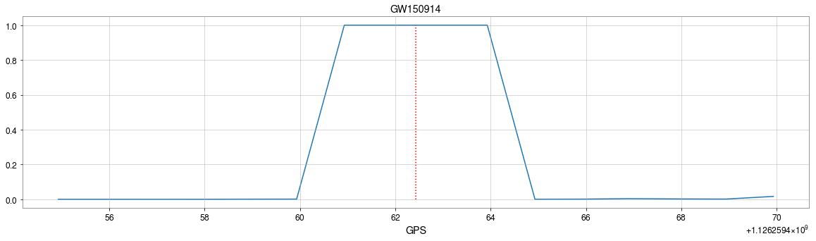
GW150914
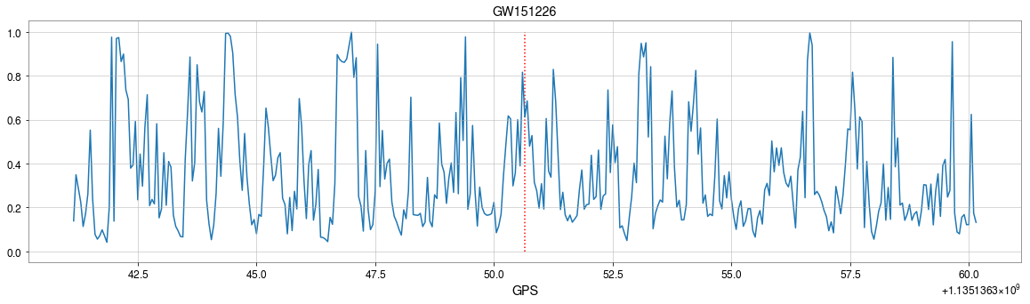
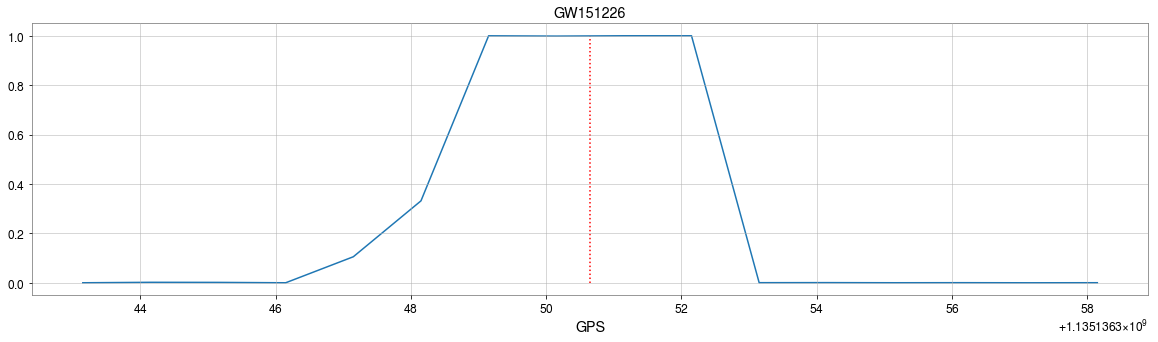
GW151226
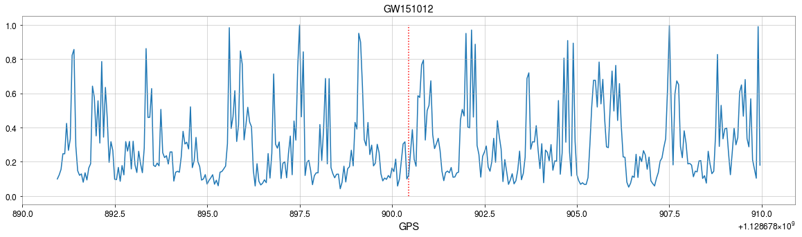
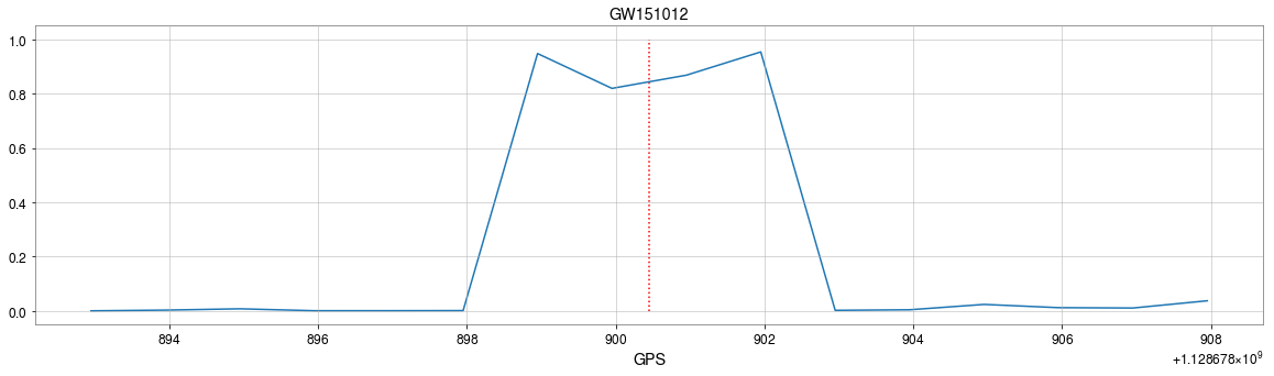
GW151012
Classification
Feature extraction
Convolutional Neural Network (ConvNet or CNN)
MFCNN
MFCNN
MFCNN
Classification
Feature extraction
Convolutional Neural Network (ConvNet or CNN)
A specific design of the architecture is needed.
GW150914
GW151226
GW151012
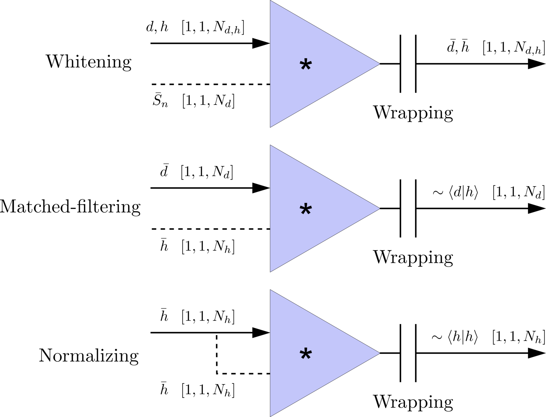
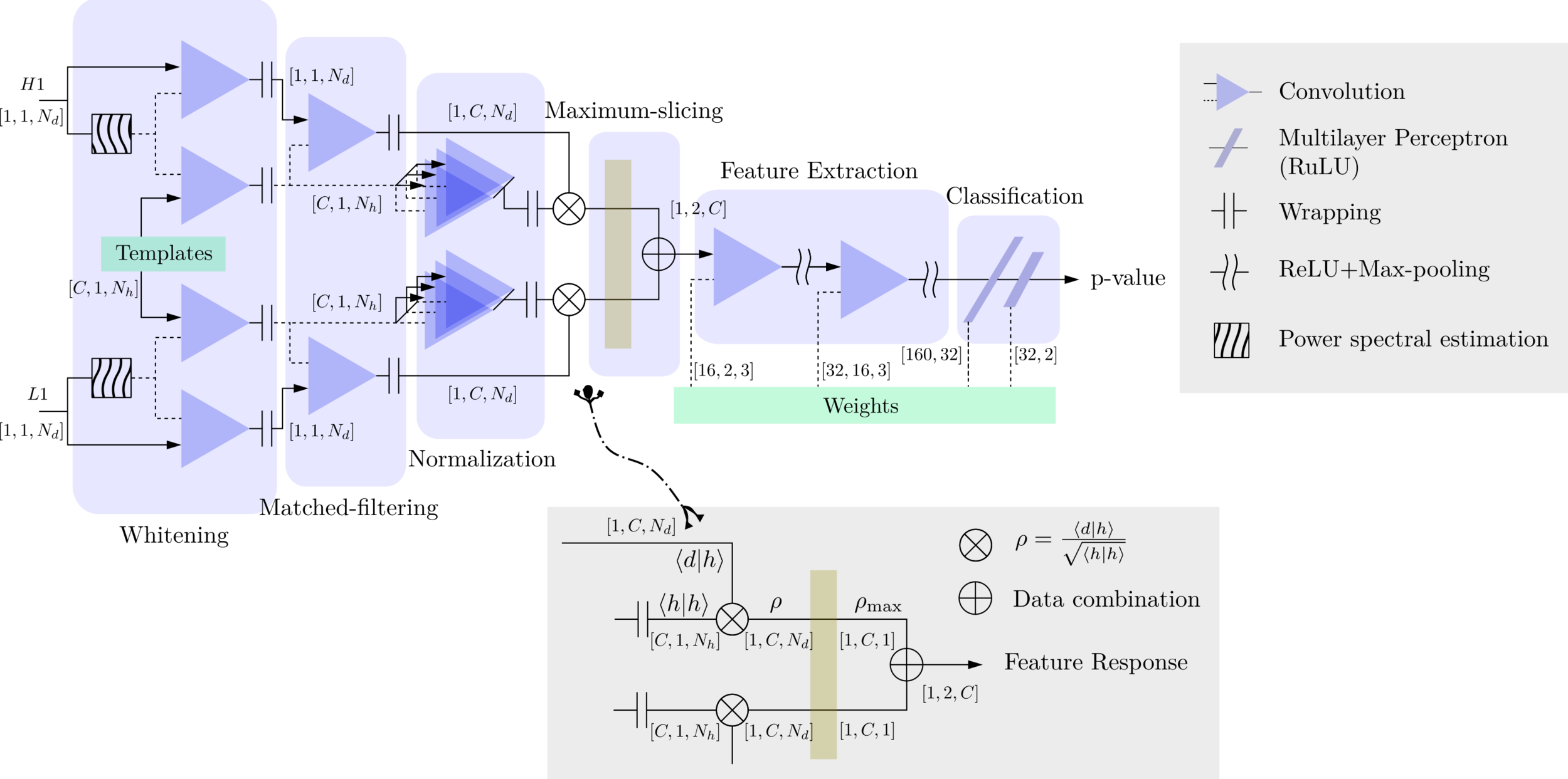
Matched-filtering (cross-correlation with the templates) can be regarded as a convolutional layer with a set of predefined kernels.
>> Is it matched-filtering ?
>> Wait, It can be matched-filtering!
Classification
Feature extraction
Convolutional Neural Network (ConvNet or CNN)
\(S_n(|f|)\) is the one-sided average PSD of \(d(t)\)
(whitening)
where
Time domain
Frequency domain
(normalizing)
(matched-filtering)
Deep Learning Framework
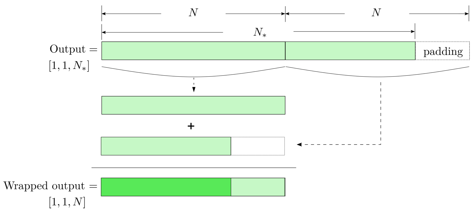
modulo-N circular convolution
\(S_n(|f|)\) is the one-sided average PSD of \(d(t)\)
(whitening)
where
Time domain
Frequency domain
(normalizing)
(matched-filtering)
FYI: \(N_\ast = \lfloor(N-K+2P)/S\rfloor+1\)
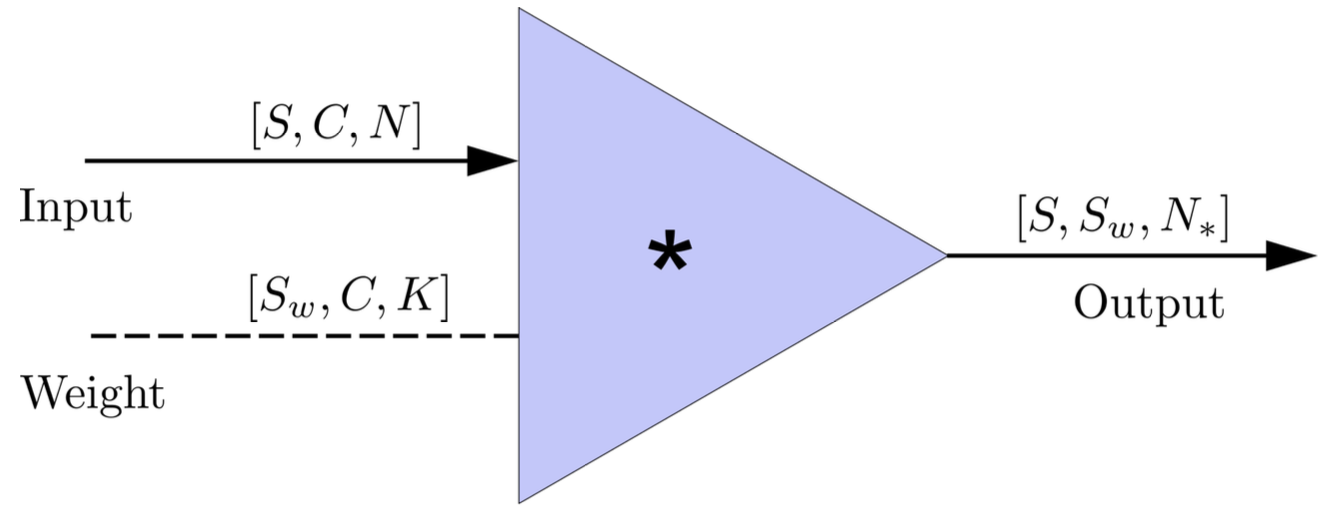
(A schematic illustration for a unit of convolution layer)
Deep Learning Framework
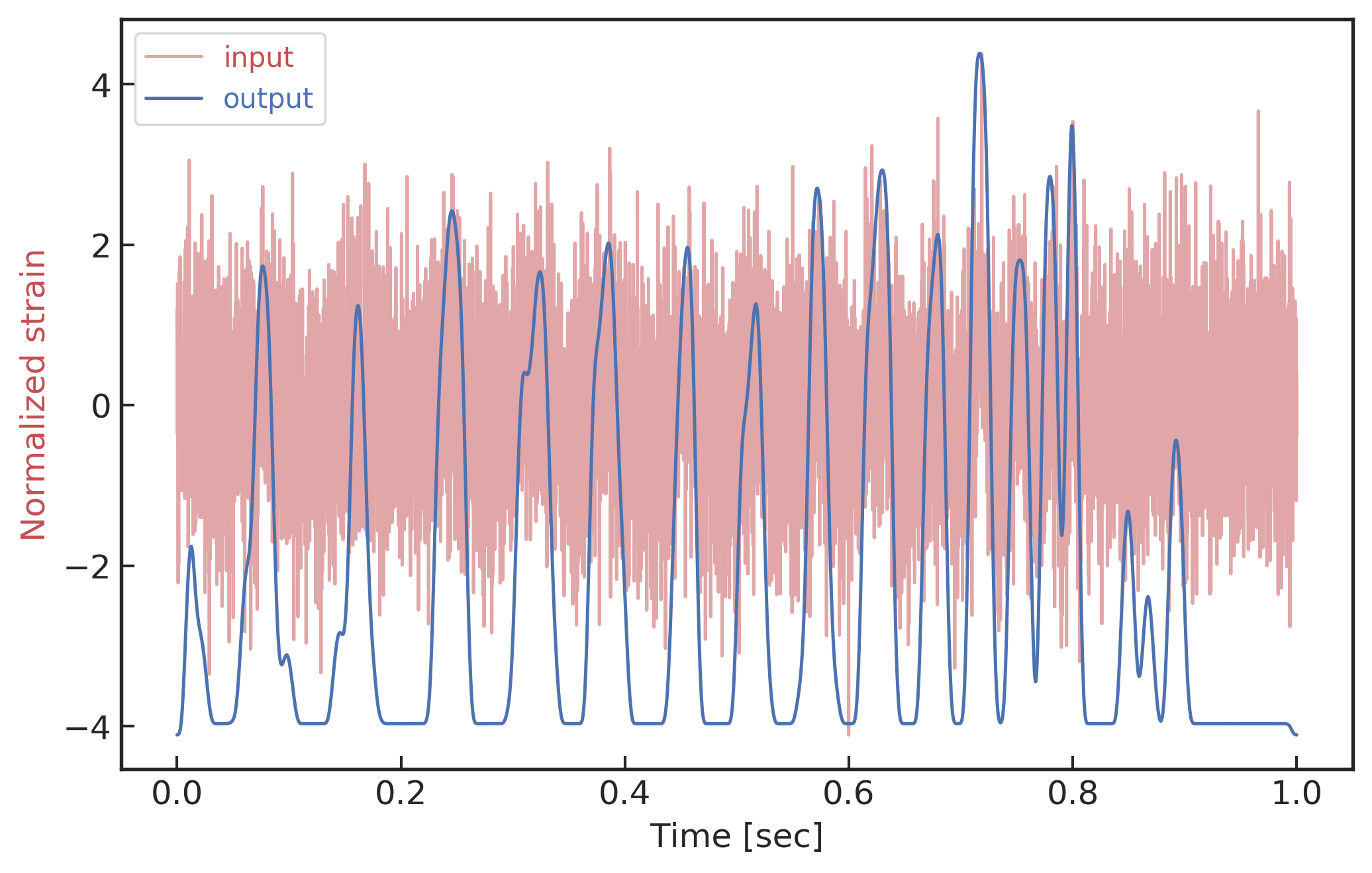
Input
Output
Input
Output
import mxnet as mx
from mxnet import nd, gluon
from loguru import logger

def MFCNN(fs, T, C, ctx, template_block, margin, learning_rate=0.003):
    logger.success('Loading MFCNN network!')
    net = gluon.nn.Sequential()
    with net.name_scope():
        net.add(MatchedFilteringLayer(mod=fs*T, fs=fs,
                                      template_H1=template_block[:,:1],
                                      template_L1=template_block[:,-1:]))
        net.add(CutHybridLayer(margin = margin))
        net.add(Conv2D(channels=16, kernel_size=(1, 3), activation='relu'))
        net.add(MaxPool2D(pool_size=(1, 4), strides=2))
        net.add(Conv2D(channels=32, kernel_size=(1, 3), activation='relu'))
        net.add(MaxPool2D(pool_size=(1, 4), strides=2))
        net.add(Flatten())
        net.add(Dense(32))
        net.add(Activation('relu'))
        net.add(Dense(2))
	# Initialize parameters of all layers
    net.initialize(mx.init.Xavier(magnitude=2.24), ctx=ctx, force_reinit=True)
    return net
The available codes: https://gist.github.com/iphysresearch/a00009c1eede565090dbd29b18ae982c
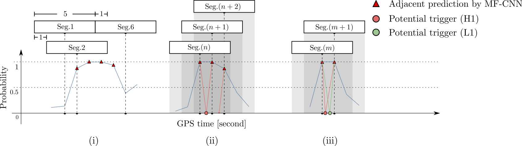
1 sec duration
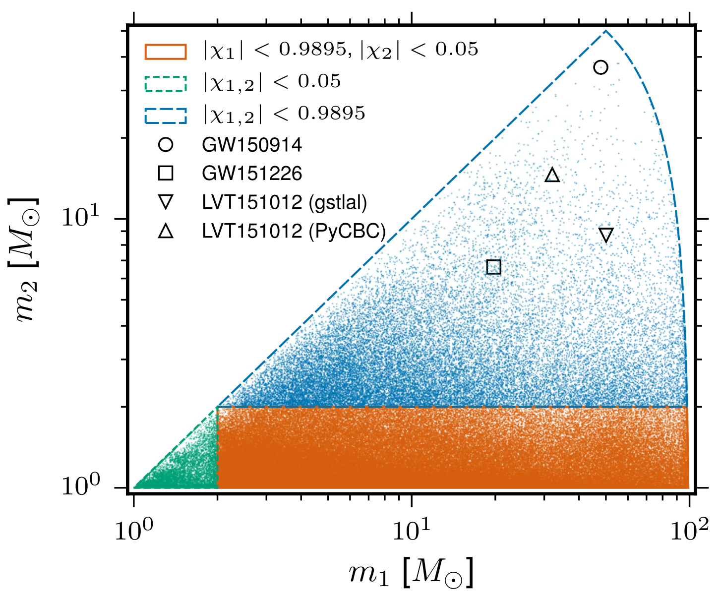
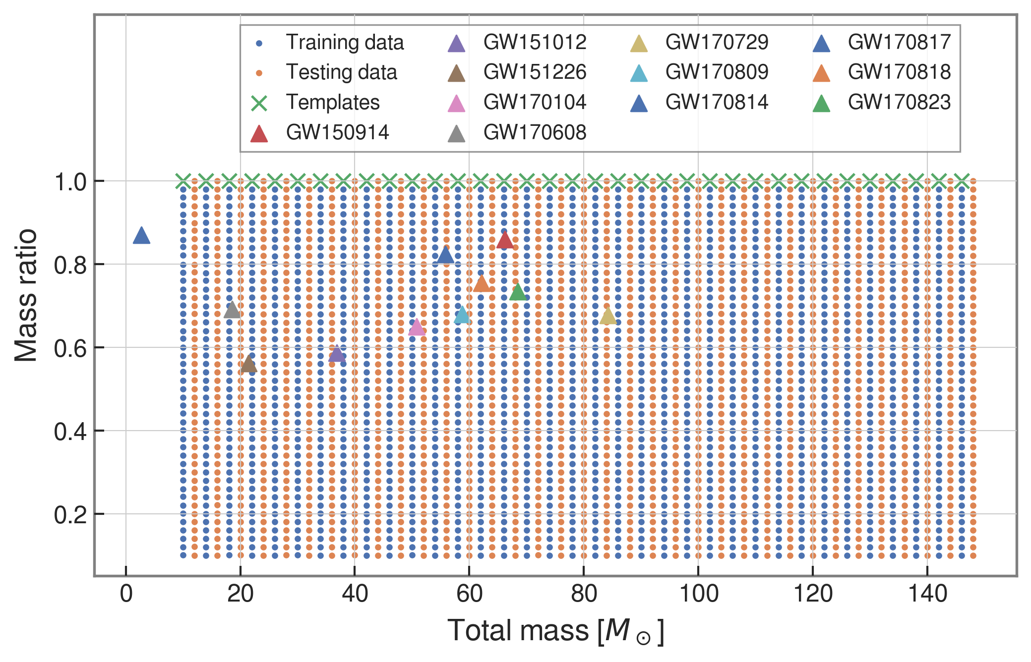
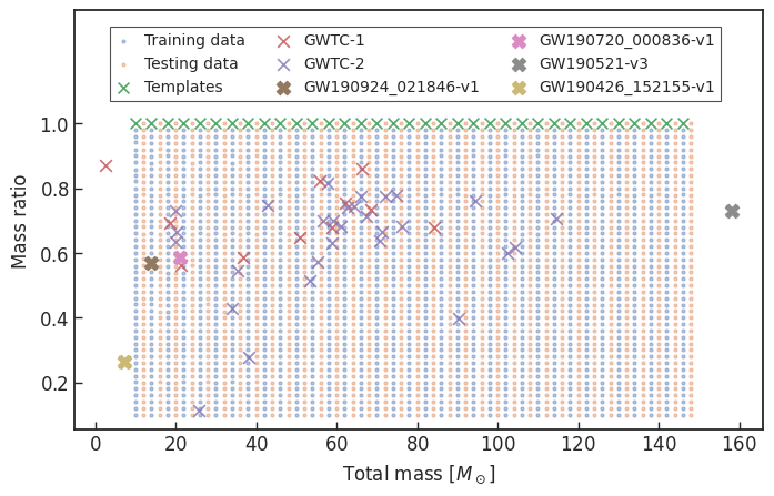
35 templates used
FYI: sampling rate = 4096Hz
| templates | waveforms (train/test) | |
|---|---|---|
| Number | 35 | 1610 |
| Length (sec) | 1 | 5 |
| equal mass |
input
GW170817
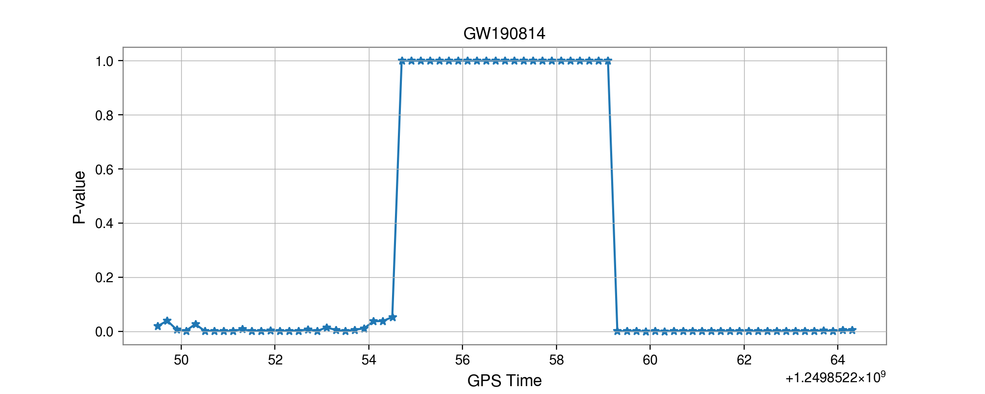
GW190814
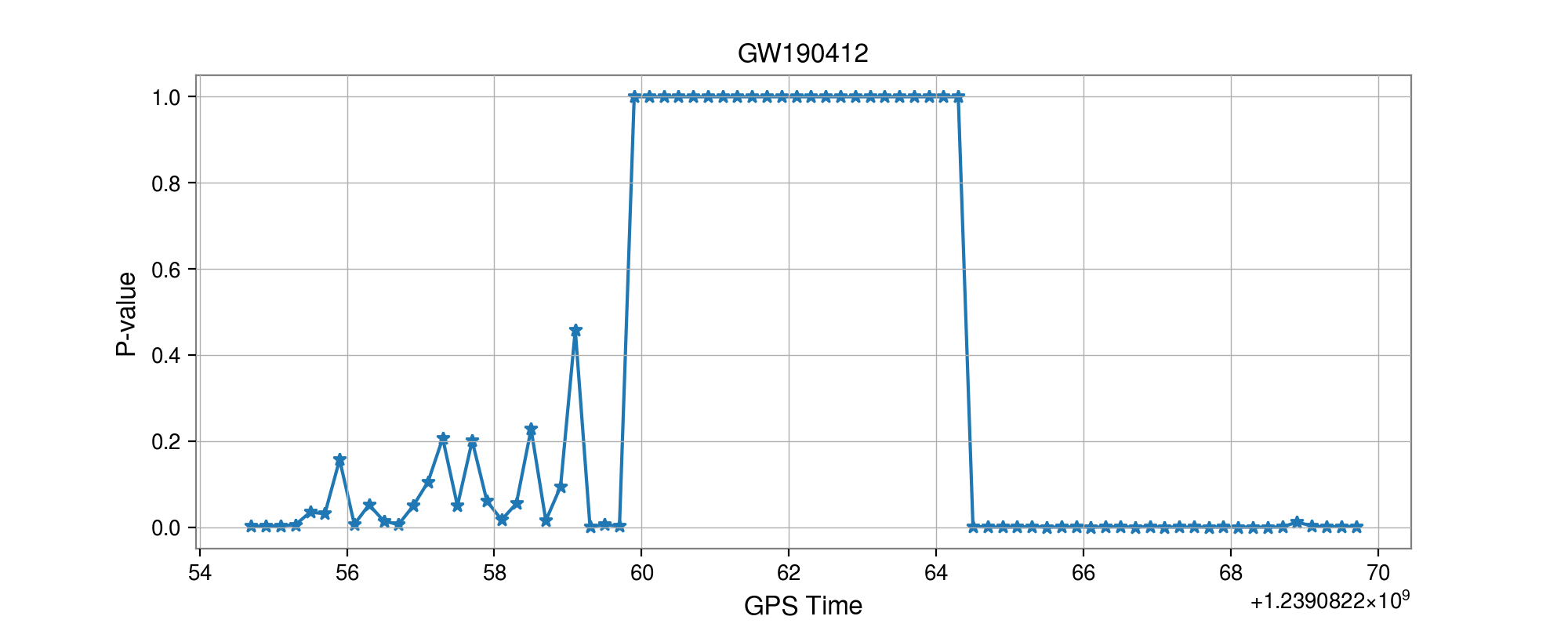
GW190412
GW170817
GW190814
GW190412
Proof-of-principle studies
Production search studies
Current paradigm:
More related works, see 2005.03745 or Survey4GWML (https://iphysresearch.github.io/Survey4GWML/)
Last updated on April. 2021
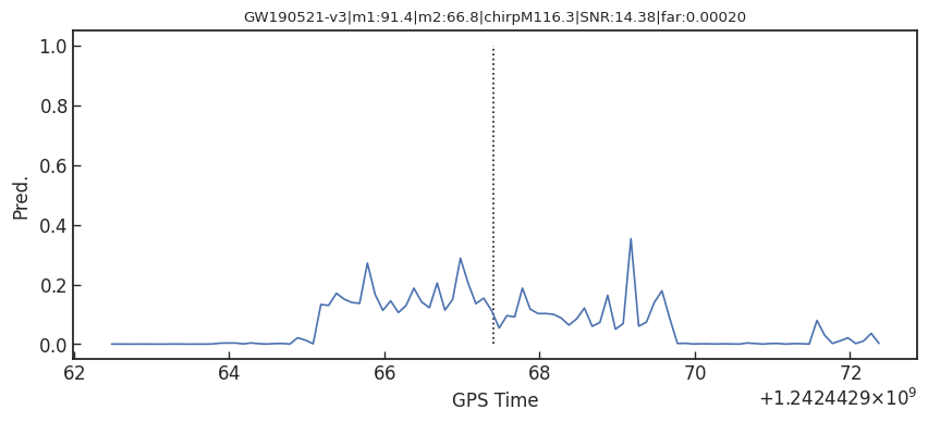
Drawbacks:
Softmax function
Score
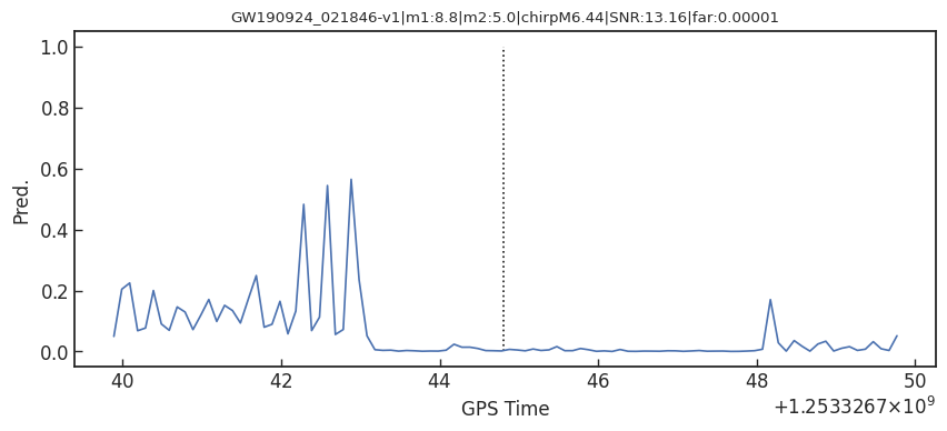
Pred.
Noise
Noise + Signal
Pred.
Possible ways to resolve the problem:
Detection of early inspiral of GW
for _ in range(num_of_audiences):
    print('Thank you for your attention! 🙏')
This slide: https://slides.com/iphysresearch/gra2020-2021
Proof-of-principle studies
Production search studies
Current paradigm:
More related works, see 2005.03745 or Survey4GWML (https://iphysresearch.github.io/Survey4GWML/)
Last updated on April. 2021
Drawbacks:
Softmax function
Score
Pred.
Noise
Noise + Signal
Pred.
Possible ways to resolve the problem:
Detection of early inspiral of GW
By He Wang
中国物理学会引力与相对论天体物理分会 , 14:40-15:00 on April 24th, 2021


