Video from:
Kehrle, F., et. al. (2011), Optimal control of formula 1 race cars in a VDrift based virtual environment
Real-Time Iterations and Multi-Level Iterations
Ihno Schrot, Heidelberg University
MORFAE Workshop at BOSCH Renningen on March 08, 2024
OUTLINE
1
Optimal Control Problem Formulation and Nonlinear Model Predictive Control
2
Problem Discretization using Direct Multiple Shooting
3
The Sequential Quadratic Programming Method as Solution Method for the Nonlinear Programs
4
Real - Time Iterations
5
Multi - Level Iterations
1
Optimal Control Problem Formulation and Nonlinear Model Predictive Control
Ihno Schrot — Real-Time Iterations and Multi-Level Iterations — MORFAE Workshop Renningen — March 08, 2024
Objective Function
Dynamical System
Continuous Constraints
Terminal Constraints
State $$x$$
Control $$u$$
Parameter $$p$$
1. OCP AND NMPC
Ihno Schrot — Real-Time Iterations and Multi-Level Iterations — MORFAE Workshop Renningen — March 08, 2024
1. OCP AND NMPC
Ihno Schrot — Real-Time Iterations and Multi-Level Iterations — MORFAE Workshop Renningen — March 08, 2024
\(x\): States
1. OCP AND NMPC
Ihno Schrot — Real-Time Iterations and Multi-Level Iterations — MORFAE Workshop Renningen — March 08, 2024
1. OCP AND NMPC
\(x\): States
\(u\): Controls
Ihno Schrot — Real-Time Iterations and Multi-Level Iterations — MORFAE Workshop Renningen — March 08, 2024
1. OCP AND NMPC
\(x\): States
\(u\): Controls
\(p\): Parameters
Ihno Schrot — Real-Time Iterations and Multi-Level Iterations — MORFAE Workshop Renningen — March 08, 2024
1. OCP AND NMPC
\(x\): States
\(u\): Controls
\(p\): Parameters
Ihno Schrot — Real-Time Iterations and Multi-Level Iterations — MORFAE Workshop Renningen — March 08, 2024
1. OCP AND NMPC
\(x\): States
\(u\): Controls
\(p\): Parameters
Ihno Schrot — Real-Time Iterations and Multi-Level Iterations — MORFAE Workshop Renningen — March 08, 2024
1. OCP AND NMPC
\(x\): States
\(u\): Controls
\(p\): Parameters
Ihno Schrot — Real-Time Iterations and Multi-Level Iterations — MORFAE Workshop Renningen — March 08, 2024
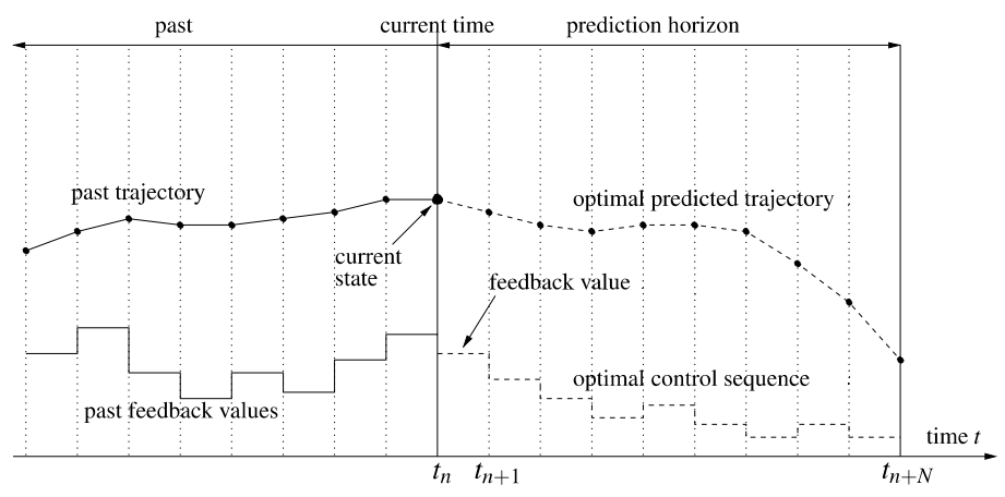
1. Measure current state $$x_k$$
Repeat:
Illustration based on Grüne and Pannek, Nonlinear Model Predictive Control
1. OCP AND NMPC
Ihno Schrot — Real-Time Iterations and Multi-Level Iterations — MORFAE Workshop Renningen — March 08, 2024
2. Solve OCP for horizon $$[t_k,t_k+T]$$
1. Measure current state $$x_k$$
Repeat:
Illustration based on Grüne and Pannek, Nonlinear Model Predictive Control
1. OCP AND NMPC
Ihno Schrot — Real-Time Iterations and Multi-Level Iterations — MORFAE Workshop Renningen — March 08, 2024
2. Solve OCP for horizon $$[t_k,t_k+T]$$
1. Measure current state $$x_k$$
3. Apply first part of computed contol
4. Progress to time $$t_{k+1}$$
Repeat:
Illustration based on Grüne and Pannek, Nonlinear Model Predictive Control
1. OCP AND NMPC
Ihno Schrot — Real-Time Iterations and Multi-Level Iterations — MORFAE Workshop Renningen — March 08, 2024
Illustration based on Grüne and Pannek, Nonlinear Model Predictive Control
1. OCP AND NMPC
2. Solve OCP for horizon $$[t_k,t_k+T]$$
4. Progress to time $$t_{k+1}$$
1. Measure current state \(x_k\)
3. Apply first part of computed contol
Ihno Schrot — Real-Time Iterations and Multi-Level Iterations — MORFAE Workshop Renningen — March 08, 2024
1. OCP AND NMPC
Ihno Schrot — Real-Time Iterations and Multi-Level Iterations — MORFAE Workshop Renningen — March 08, 2024
OUTLINE
1
Optimal Control Problem Formulation and Nonlinear Model Predictive Control
2
Problem Discretization using Direct Multiple Shooting
3
The Sequential Quadratic Programming Method as Solution Method for the Nonlinear Programs
4
Real - Time Iterations
5
Multi - Level Iterations
Ihno Schrot — Real-Time Iterations and Multi-Level Iterations — MORFAE Workshop Renningen — March 08, 2024
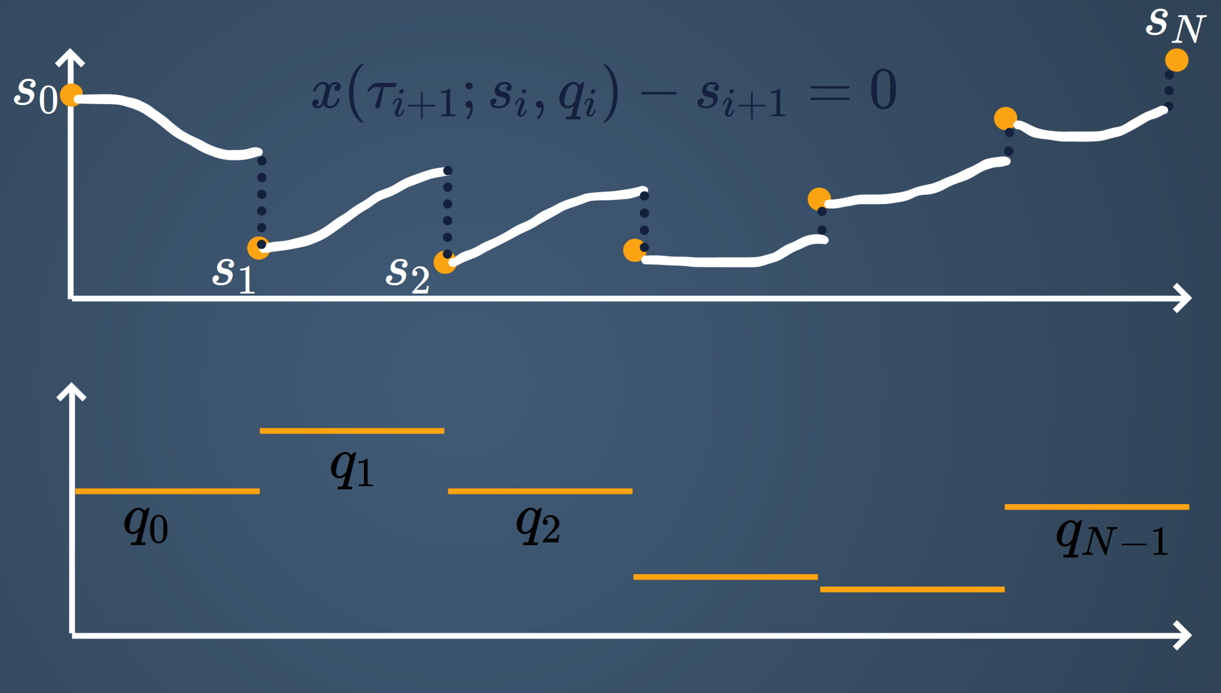
1. Introduce Shooting Grid
State $$x(\cdot)$$
Control $$u(\cdot)$$
2. Replace state trajectory by points
3. Replace control trajectory by, e.g., piecewise constant controls
4. Introduce Matching Conditions

Infinite-Dimensional
Bock, H. G., & Plitt, K. J. (1984). A multiple shooting algorithm for direct solution of optimal control problems.
2. MULTIPLE SHOOTING
Ihno Schrot — Real-Time Iterations and Multi-Level Iterations — MORFAE Workshop Renningen — March 08, 2024
Finite-dimensional nonlinear program
2. MULTIPLE SHOOTING
Ihno Schrot — Real-Time Iterations and Multi-Level Iterations — MORFAE Workshop Renningen — March 08, 2024
OUTLINE
1
Optimal Control Problem Formulation and Nonlinear Model Predictive Control
2
Problem Discretization using Direct Multiple Shooting
3
The Sequential Quadratic Programming Method as Solution Method for the Nonlinear Programs
4
Real - Time Iterations
5
Multi - Level Iterations
Ihno Schrot — Real-Time Iterations and Multi-Level Iterations — MORFAE Workshop Renningen — March 08, 2024
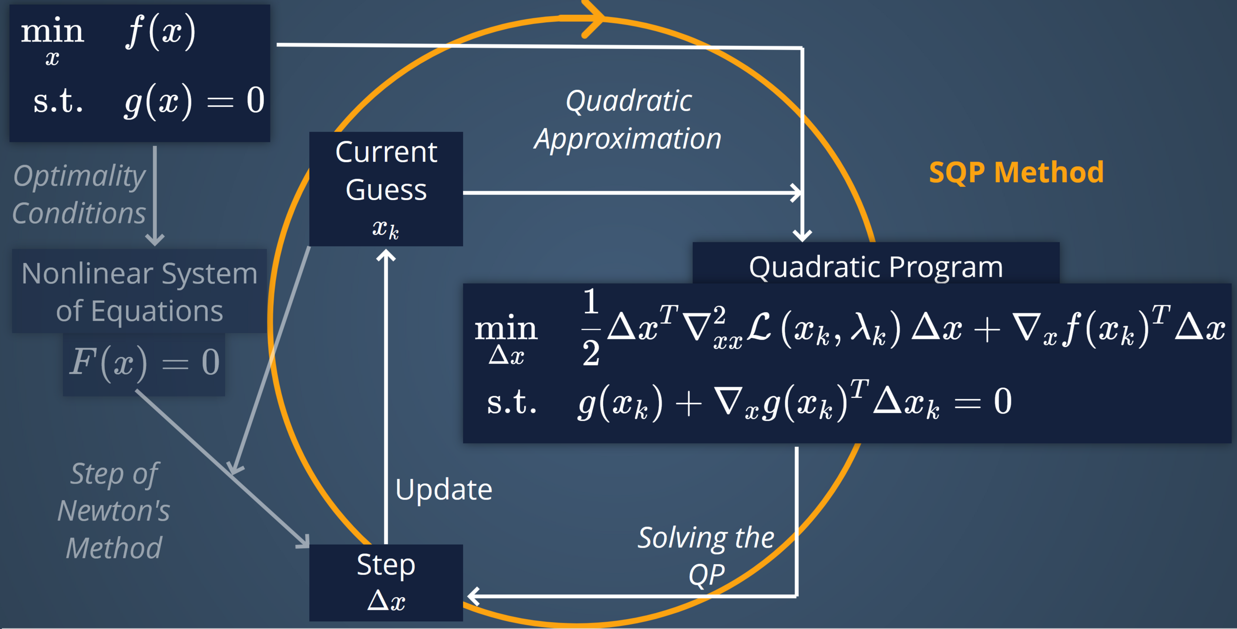
Nonlinear System of Equations
SQP Method
Step of Newton's Method
Optimality Conditions
Quadratic Approximation
Quadratic Program
Step $$\Delta x$$
Current Guess $$x_k$$
Solving the QP
Update
3. SQP METHOD
Ihno Schrot — Real-Time Iterations and Multi-Level Iterations — MORFAE Workshop Renningen — March 08, 2024
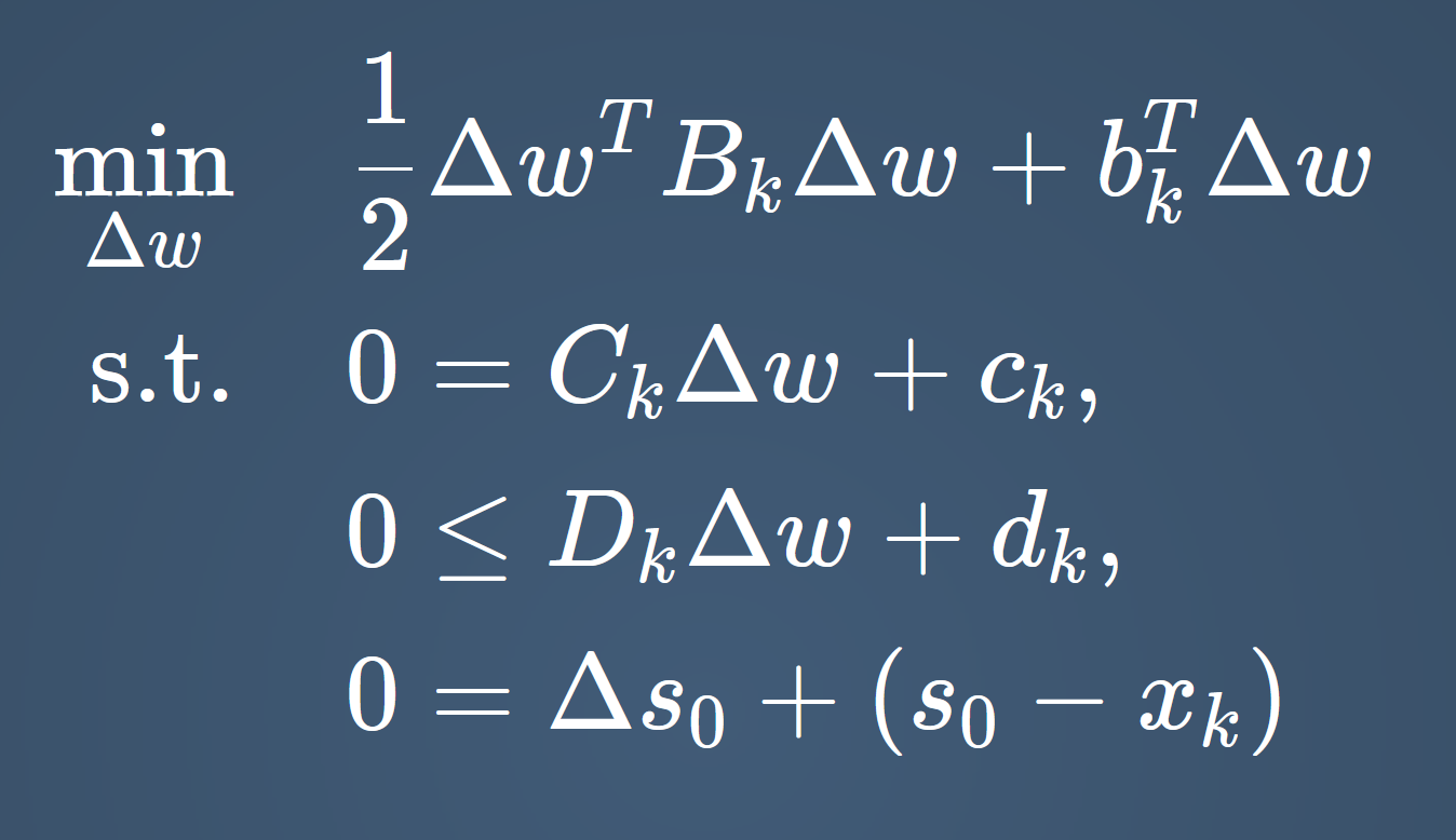
In the case of Multiple Shooting:
- QPs are highly structured
- QPs can be condensed so that they only depend on \(\Delta s_0, \Delta q_0,\ldots,\Delta q_{N-1} \)
\(\Delta w \): (Primal) Variables including \(\Delta s_0 \)
\(B_k \): Hessian of Lagrangian
\(b_k \): Objective gradient
\(C_k, D_k \): Jacobians of (in-)equality constraints
\(c_k, d_k \): Residuals of (in-)equality constraints
QP at sampling time \(t_k\):
3. SQP METHOD
Initial Value Embedding Constraint
Depend only on \(w_k\)
Ihno Schrot — Real-Time Iterations and Multi-Level Iterations — MORFAE Workshop Renningen — March 08, 2024
OUTLINE
1
Optimal Control Problem Formulation and Nonlinear Model Predictive Control
2
Problem Discretization using Direct Multiple Shooting
3
The Sequential Quadratic Programming Method as Solution Method for the Nonlinear Programs
4
Real - Time Iterations
5
Multi - Level Iterations
Ihno Schrot — Real-Time Iterations and Multi-Level Iterations — MORFAE Workshop Renningen — March 08, 2024
Observations:
- Exact controls cannot be computed without delay
\(\rightarrow\) Rather compute approximate solutions quickly! - Subsequent OCPs parametrized by current state \(x_k\)
Efficient solution method: Parametric Active-Set Method implemented in qpOASES
Diehl, M., et. al. (2002). Real-time optimization and nonlinear model predictive control of processes governed by differential-algebraic equations.
1st key idea of RTI:
Perform only a single SQP iteration per sample time
Solve:
Ferreau, H. J., et. al. (2014). qpOASES: A parametric active-set algorithm for quadratic programming.
4. REAL-TIME ITERATIONS
Ihno Schrot — Real-Time Iterations and Multi-Level Iterations — MORFAE Workshop Renningen — March 08, 2024
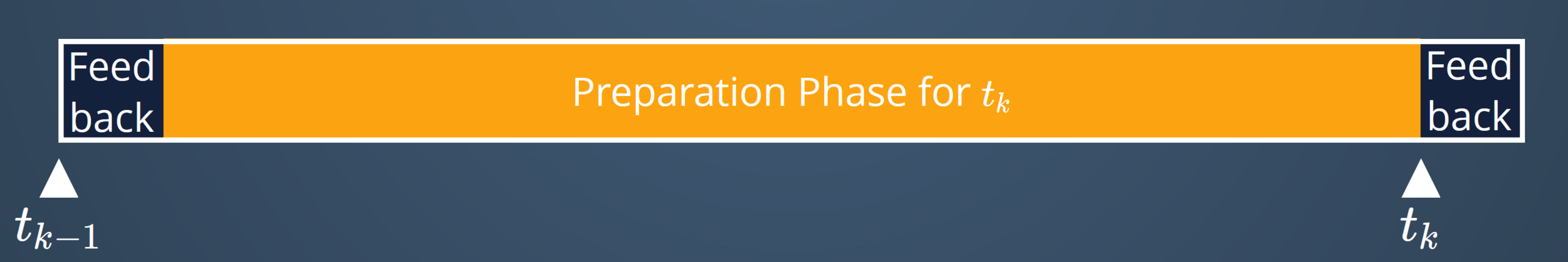
Observation: Current state \(x_k\) enters OCPs linearly
2nd key idea of RTI:
Split computations in preparation and feedback phase
Preparation Phase for \(t_k\)
Feedback
Feedback
4. REAL-TIME ITERATIONS
Ihno Schrot — Real-Time Iterations and Multi-Level Iterations — MORFAE Workshop Renningen — March 08, 2024
OUTLINE
1
Optimal Control Problem Formulation and Nonlinear Model Predictive Control
2
Problem Discretization using Direct Multiple Shooting
3
The Sequential Quadratic Programming Method as Solution Method for the Nonlinear Programs
4
Real - Time Iterations
5
Multi - Level Iterations
Ihno Schrot — Real-Time Iterations and Multi-Level Iterations — MORFAE Workshop Renningen — March 08, 2024
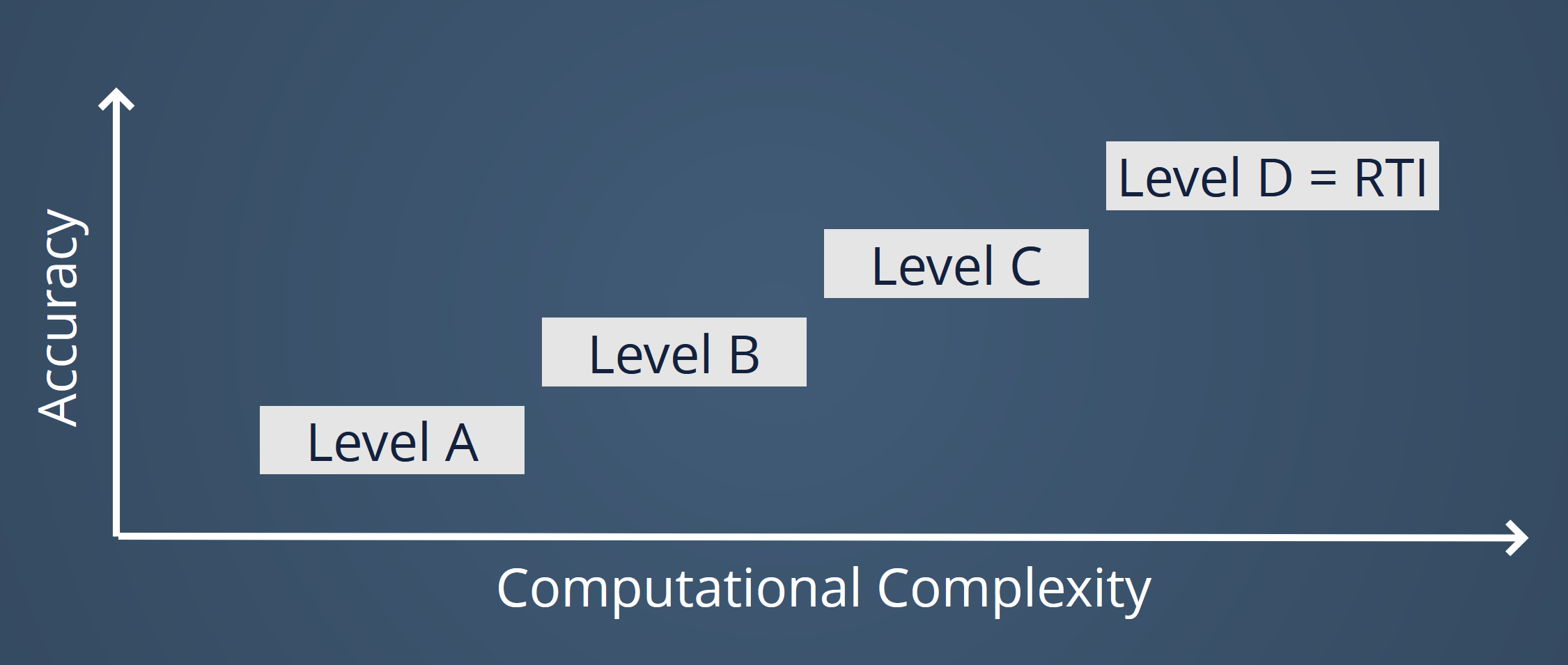
Observation: Linearizations can be valid for a longer time period
Key idea of MLI:
Reduce expensive evaluations by updating the QPs in 4 levels
Wirsching, L. (2018). Multi-Level Iteration Schemes with Adaptive Level Choice for Nonlinear Model Predictive Control.
Level D = RTI
Level C
Level B
Level A
Computational Complexity
Accuracy
Level D = RTI
Level C
Level B
Level A
Levels can run in parallel and communicate with each other.
5. MULTI-LEVEL ITERATIONS
Ihno Schrot — Real-Time Iterations and Multi-Level Iterations — MORFAE Workshop Renningen — March 08, 2024
Level D = RTI
Computational Complexity
Accuracy
Level D = RTI
Level C
Level B
Level A
Level C
Level B
Level A
5. MULTI-LEVEL ITERATIONS
Ihno Schrot — Real-Time Iterations and Multi-Level Iterations — MORFAE Workshop Renningen — March 08, 2024
Computational Complexity
Accuracy
Level D = RTI
Level C
Level B
Level A
Level D = RTI
Level D = RTI
Level C
Level B
Level A
Full linearization iterations
5. MULTI-LEVEL ITERATIONS
Ihno Schrot — Real-Time Iterations and Multi-Level Iterations — MORFAE Workshop Renningen — March 08, 2024
Computational Complexity
Accuracy
Level D = RTI
Level C
Level B
Level A
Level D = RTI
Level D = RTI
Full linearization iterations
Level C
Level B
Level A
Optimality Iterations
No new Hessian and (full) Jacobians!
New Jacobians enter as matrix-vector products only
5. MULTI-LEVEL ITERATIONS
Ihno Schrot — Real-Time Iterations and Multi-Level Iterations — MORFAE Workshop Renningen — March 08, 2024
Computational Complexity
Accuracy
Level D = RTI
Level C
Level B
Level A
Level D = RTI
Level D = RTI
Full linearization iterations
Level C
Level B
Level A
Optimality Iterations
Feasibility Iterations
No new Jacobians involved
5. MULTI-LEVEL ITERATIONS
Ihno Schrot — Real-Time Iterations and Multi-Level Iterations — MORFAE Workshop Renningen — March 08, 2024
Computational Complexity
Accuracy
Level D = RTI
Level C
Level B
Level A
Level D = RTI
Level D = RTI
Full linearization iterations
Level C
Level B
Level A
Optimality Iterations
Feasibility Iterations
Feedback Iterations
5. MULTI-LEVEL ITERATIONS
Ihno Schrot — Real-Time Iterations and Multi-Level Iterations — MORFAE Workshop Renningen — March 08, 2024
4. MLI: Reduce expensive evaluations by updating the QPs in 4 levels
3. RTI: Solve only one QP per sampling time and split computations in preparation and feedback phase
2. Apply an SQP-type method to the NLPs
1. The \(\infty\)-dim. OCP is discretized using Multiple Shooting
SUMMARY
Ihno Schrot — Real-Time Iterations and Multi-Level Iterations — MORFAE Workshop Renningen — March 08, 2024
4. REAL-TIME ITERATIONS
Ihno Schrot — Real-Time Iterations and Multi-Level Iterations — MORFAE Workshop Renningen — March 08, 2024
5. MULTI-LEVEL ITERATIONS
Uncontrolled chain
Chain controlled with MLI
Videos from: Wirsching, L. (2018). Multi-Level Iteration Schemes with Adaptive Level Choice for Nonlinear Model Predictive Control.
Ihno Schrot — Real-Time Iterations and Multi-Level Iterations — MORFAE Workshop Renningen — March 08, 2024