Aim 3: Posterior Sampling and Uncertainty


September 20, 2022

Problem Statement (refresher)

y = x + v_0,~v_0 \sim \mathcal{N}(0, \sigma_0^2 \mathbb{I})

retrieval of \(x\) is ill-posed

\hat{x} \sim p(x \mid y)

sample \(\hat{x}\) without access to \(p(x)\)

A Brief History on Langevin Dynamics

3. [Kadkhodaie, 21] \(\mathbb{E}[x \mid \tilde{x}] = \tilde{x} + \sigma^2 \nabla_x \log~p(x)\)

0. Langevin diffusion equation

x_{t+1} = x_t - \alpha \nabla U(x_t) + \sqrt{2\alpha}z_t

2. [Song, 19 & 21] Noise Conditional Score Networks

U(x) = -\log~p(x),~\nabla_x \log~p(x_t) \approx s(\theta^*, \sigma)\\ \theta^* = \arg \min \mathbb{E}_{(x,~\tilde{x} \sim \mathcal{N}(x, \{\sigma_i\}_{i=1}^L\mathbb{I}))} [\|\sigma s_\theta(x, \sigma) + \frac{\tilde{x} - x}{\sigma^2}\|^2]

4. [Kawar, 21] Stochastic Denoising

\tilde{x}_{t+1} = \tilde{x}_t + \alpha \nabla_x \log~p(\tilde{x}_t \mid y) + \sqrt{2\alpha}z_t\\ \nabla_x \log~p(\tilde{x}_t \mid y) = s_{\theta^*}(x, \sigma_t) + \frac{y - \tilde{x}_t}{\sigma_0^2 - \sigma_i^2}

Stochastic Denoising With an NCSN 

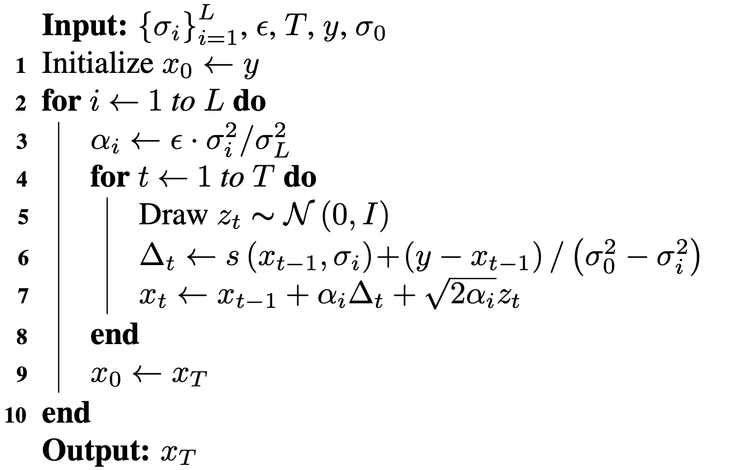
Algorithm 1: Stochastic image denoiser, [Kawar, 21]

Training an NCSN on Abdomen CT - I

Data: AbdomenCT-1K [GitHub] [paper]

\(\approx 170 \times 10^3\) train / \(\approx 40 \times 10^3\) val images, \(256 \times 256\) pixels

Figure 2: Some example images from the validation split.

Figure 1: Some augmented example images from the training split.

Training an NCSN on Abdomen CT - II

Model: U-net based on NCSNv2 [GitHub] [paper]

Noise scales: \(\{\sigma_i\}_{i=1}^L,~\sigma_1 > \sigma_2 > ... > \sigma_L = 0.01\)

\sigma_1 \approx \max_{(x, x') \in S_{\text{train}}} \|x - x'\|_2 \approx 124,\\ \frac{\sigma_i}{\sigma_{i+1}} = \gamma \approx 1.008356 \implies L \approx 1183

(from Song, 21)

Hardware: 8 NVIDIA RTX A5000 (24 GB of RAM each)

Preliminary Sampling Results - I

We set \(\epsilon = 1 \times 10^{-6},~T = 3\) in Algorithm 1

Original

Sampled

\(\sigma_0 = 0.1\)

Perturbed

Preliminary Sampling Results - II

We set \(\epsilon = 1 \times 10^{-6},~T = 3\) in Algorithm 1

Original

Sampled

\(\sigma_0 = 0.2\)

Perturbed

Preliminary Sampling Results - III

We set \(\epsilon = 1 \times 10^{-6},~T = 3\) in Algorithm 1

Sampled

\(\sigma_0 = 0.1\)

Perturbed

\(\sigma_0 = 0.2\)

\(\sigma_0 = 0.3\)

\(\sigma_0 = 0.4\)

Original

Preliminary Sampling Results - IV

Sampled

Perturbed

Preliminary Sampling Results - III

We sample \(8\) times for \(128\) validation images

Next Steps: Score SDE

0. Ito process

\text{d}x = f(x, t)\text{d}t + g(t)\text{d}w

1. [Anderson, 82] Reverse-time SDE

\text{d}x = [f(x, t) - g^2(t)~\nabla_x \log~p_t(x)]\text{d}t + g(t)\text{d}\bar{w}

\(\implies\)

2. [Song, 21] SDE Score Network

\theta^* = \arg \min \mathbb{E}_{(t,~x(0),~x(t) \mid x(0))}\left[\| s_\theta(x(t), t) - \nabla_x \log~p_{0t}(x(t)\mid x(0))\|_2^2\right]

Denoising Reverse-time SDE

\text{d}x = \sqrt{\frac{\text{d}}{\text{d}t}\sigma^2(t)} \text{d}w,~\sigma(t) = \sigma_m \cdot \left(\frac{\sigma_M}{\sigma_m}\right)^t\\ x_t = x_{t + 1} + \sigma^2(t + 1) \left[s_{\theta^*}(x_{t+1}, t + 1) + \frac{y - x_{t+1}}{\sigma^2 - \sigma^2(t + 1)}\right]~\Delta t + \sigma(t+1)z_{t+1}\sqrt{\Delta t}

Denoising Reverse-time SDE

x_t = x_{t + 1} + \sigma^2(t + 1) \left[s_{\theta^*}(x_{t+1}, t + 1) + \frac{y - x_{t+1}}{\sigma^2 - \sigma^2(t + 1)}\right]~\Delta t + \sigma(t+1)z_{t+1}\sqrt{\Delta t}

Euler-Maruyama discretization

Next Steps

1. Increase image size to 512 x 512

2. Different noise priors other than Gaussian

3. Use of a pretrained denoiser vs score network

4. Questions?

Appendix: Score Matching References

1. Hyvärinen, A. and Dayan, P., 2005. Estimation of non-normalized statistical models by score matching. Journal of Machine Learning Research, 6(4). [paper]

2. Vincent, P., 2011. A connection between score matching and denoising autoencoders. Neural computation23(7), pp.1661-1674. [paper]

Made with Slides.com