Overview

• Brief overview of stochastic thermodynamics

• Non-linear stochastic thermodnyamics

Thermodynamics

Microscopic systems

Classical mechanics (QM,...)

Mesoscopic systems

Stochastic thermodynamics

Macroscopic systems

Thermodynamics

Stochastic Thermodynamics is a thermodynamic theory
for mesoscopic, non-equilibrium physical systems
interacting with equilibrium thermal (and/or chemical)
reservoirs

Historical review  of thermodynamics

History

Equilibrium thermodynamics (19 th century)

- Maxwell, Boltzman, Planck, Claussius, Gibbs...

- Macroscopic systems ($N \rightarrow \infty$) in equilibrium (no time dependence of measurable quantities - thermoSTATICS)

-  General structure of thermodynamics

• Laws of thermodynamics (general)
• Response coefficients (system-specific)                               

- Applications: engines, refridgerators, air-condition,... 

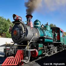
efficiency $\leq 1-\frac{T_2}{T_1}$

Heat engine: Carnot cycle

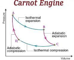
Car engines: 30-50%

History

Laws of thermodynamics

Zeroth law:

Temperature can be measured. $$T_A = T_B \quad \mathrm{if} \quad A \ \mathrm{and} \ B \ \mathrm{are} \ \mathrm{in} \ \mathrm{equilibrium}.$$

First law (Claussius 1850, Helmholtz 1847):

Energy is conserved.
$${\color{aqua} d}U = {\color{orange} \delta} Q - {\color{orange} \delta} W$$ Second law (Carnot 1824, Claussius 1854, Kelvin):

Heat cannot be fully transformed into work. $${ \color{aqua} d} S \geq \frac{{\color{orange} \delta} Q}{T}$$ Third law: We cannot bring the system into the absolute zero
temperature in a finite number of steps. $$\lim_{T \rightarrow 0} S(T) = 0$$

History

Local equilibrium thermodynamics (1st half of 1900s)

- Onsager, Rayleigh...

- Systems close to equilibrium - linear response theory

-  Local equilibrium: subsystems a,b,c are each in equilibrium  

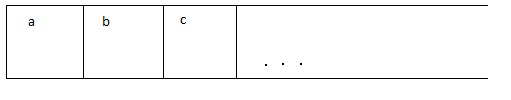
Total entropy $S \approx S^a + S^b + S^c + \dots$

Entropy production $\sigma^a = \frac{d S^a}{d t} = \sum_i Y_i^a J_i^a$

$Y_i^a$ - thermodynamic forces; $J_i^a$ - thermodynamic currents

4th Law of thermodynamics (Onsager 1931): $\sigma = \sum_{ij} L_{ij} \Gamma_i \Gamma_j$

 $\Gamma_i = Y_i^a - Y_i^b$ - afinity, $L_{ij}$ - symmetric

Molecular motor: myosin walking on actin filament

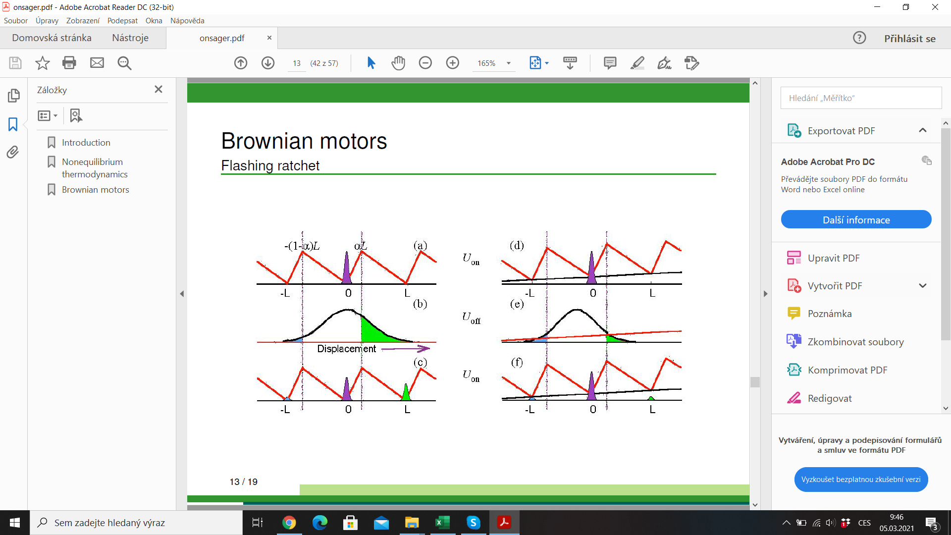
efficiency $\lesssim 1$

Main results of stochastic thermodynamics

Stochastic thermodynamics

1.) Consider linear Markov (= memoryless) with distribution $p_i(t)$.

Its evolution is described by master equation

$$\dot{p}_i(t) = \sum_{j} [w_{ij} p_{j}(t) - w_{ji} p_i(t) ]$$

$w_{ij}$ is transition rate. 

2.) Entropy of the system - Shannon entropy  $S(P) = - \sum_i p_i \log p_i$. Equilibrium distribution is obtained by maximization of $S(P)$ under the constraint of average energy $U(P) = \sum_i p_i \epsilon_i$

$$p_i^{eq} = \frac{1}{Z} \exp(- \beta \epsilon_i) \quad \mathrm{where} \ \beta=\frac{1}{k_B T}, Z = \sum_j \exp(-\beta \epsilon_j)$$

Stochastic thermodynamics

3.) Detailed balance - stationary state ($\dot{p}_i = 0$ ) coincides with the equilibrium state ($p_i^{eq}$). We obtain

$$\frac{w_{ij}}{w_{ji}} = \frac{p_i^{eq}}{p_j^{eq}} = e^{\beta(\epsilon_j - \epsilon_i)}$$

4.) Second law of thermodynamics: 

$$\dot{S} = - \sum_i \dot{p}_i \log p_i = \frac{1}{2} \sum_{ij} (w_{ij} p_j - w_{ji} p_i) \log \frac{p_j}{p_i}$$

$$=\underbrace{\frac{1}{2} \sum_{ij} (w_{ij} p_j - w_{ji} p_i) \log \frac{w_{ij} p_j}{w_{ji} p_i}}_{\dot{S}_i} + \underbrace{\frac{1}{2} \sum_{ij} (w_{ij} p_j - w_{ji} p_i) \log \frac{w_{ji}}{w_{ij}}}_{\dot{S}_e}$$

$\dot{S}_i \geq 0$ - entropy production rate (2nd law of TD)

$\dot{S}_e = \beta \dot{Q}$ entropy flow rate

Stochastic thermodynamics

5.) Trajectory thermodynamics - consider stochastic trajectory

$x(t)= (x_0,t_0;x_1,t_1;\dots)$. Energy $E_x = E_x(\lambda(t))$, $\lambda(t)$ - control protocol

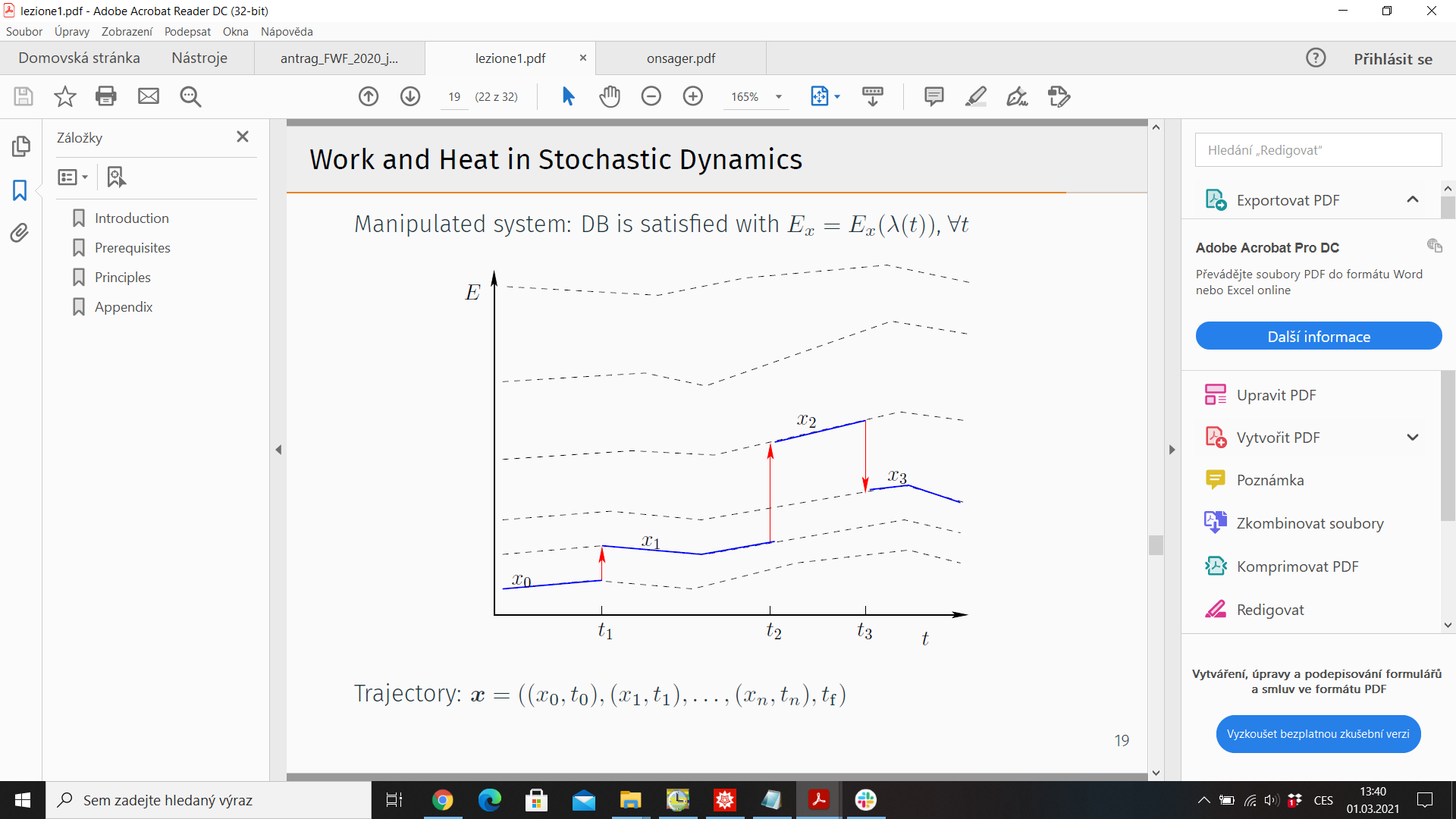
Probability of observing $x(t)$: $\mathcal{P}(x(t)$)

Time reversal $\tilde{x}(t) = x(T-t)$

Reversed protocol $\tilde{\lambda}(t) = \lambda(T-t)$

Probability of observing reversed trajectory under reversed protocol $\tilde{\mathcal{P}}(\tilde{x}(t))$

Stochastic thermodynamics

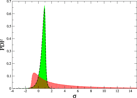
6.) Fluctuation theorems

Trajectory entropy: $s(t) = - \log p_x(t)$

Trajectory 2nd law $\Delta s = \Delta s_i + \Delta s_e$

Relation to the trajectory probabilities

$$\log \frac{\mathcal{P}(x(t))}{\tilde{\mathcal{P}}(\tilde{x}(t))} = \Delta s_i$$

Detailed fluctuation theorem

$$\frac{P(\Delta s_i)}{\tilde{P}(-\Delta s_i)} = e^{\Delta s_i}$$

Integrated fluctuation theorem $$\langle e^{- \Delta s_i} \rangle = 1 \quad \Rightarrow \langle \Delta s_i \rangle = \Delta S_i \geq 0$$

Stochastic thermodynamics for non-linear systems

Stochastic thermodynamics of       non-linear systems

(with D. Wolpert - New J. Phys.  doi:10.1088/1367-2630/abea46)

• Many complex, long-range systems are non-linear
• Question: can we use stochastic thermodynamics?

Requirements:

1. Non-linear Markov dynamics $$\dot{p}_i(t) = \frac{1}{C(p)} \sum_{j} [w_{ij} \Omega(p_{j}(t)) - w_{ji} \Omega(p_i(t)) ]$$
2. Detailed balance $$\frac{w_{ij}}{w_{ji}} = \frac{\Omega(p_i^{eq})}{\Omega(p_j^{eq})}$$
3. Second law of thermodynamics:

• ​​For some (generalized) entropy : $\dot{S}_i \geq 0$.

Generalized entropies

• Studied in information theory since 60'S​​

• used in physics since 90's​

• Main aim: study thermodynamics of systems with non-Botlzmannian equilibrium distributions  (due to correlations, long-range interactions...)

• We consider  a sum-class form of entropy:

$S(P) = f\left(\sum_m g(p_m) \right)$

• Maximum entropy principle: Maximize S(p) subject to constraint that p is normalized and expected energy has a given value

Solution: MaxEnt distribution: $p^\star_m = (g')^{-1} \left(\frac{\alpha+\beta \epsilon_m}{C_f} \right)$,         

   $C_f = f'(\sum_m g(p_m))$

Theorem: Requirements 1-3 imply

1) $\Omega(p_m) = \exp(-g'(p_m))$

2) $C(p) = f'(\sum_m g(p_m))$

Generalized entropies for non-linear systems

Corollary: 

a)     $S(p) = f\left(-\sum_m \int_0^{p_m} \log \Omega(z) \mathrm{d} z \right)$

b)      $\frac{w_{mn}}{w_{nm}} = \frac{\epsilon_m-\epsilon_n}{T}$

Sketch of proof

$\dot{S} = C_f \sum_m \dot{p}_m g'(p_m)$

   $= \frac{C_f}{2} \sum_{mn} (J_{mn}-J_{nm}) (g'(p_m) - g'(p_n))$

$= \frac{C_f}{2} \sum_{mn} (J_{mn}-J_{nm}) (\Phi_{mn} - \Phi_{nm})$

   $+ \frac{C_f}{2} \sum_{mn}  (J_{mn}-J_{nm}) (g'(p_m)+\Phi_{nm} - g'(p_n) - \Phi_{mn})$

 $= \underbrace{\frac{C_f}{2} \sum_{mn} (J_{mn}-J_{nm}) (\phi(J_{mn}) - \phi(J_{nm}) )}_{\dot{S}_i}$

$+ \underbrace{\frac{C_f}{2} \sum_{mn}  (J_{mn}-J_{nm}) (g'(p_m)+\phi(J_{nm}) - g'(p_n) - \phi(J_{mn}) )}_{\dot{S}_e}$

Sketch of proof

$\dot{S}_i \Rightarrow \phi - \ increasing$

$\dot{S}_e \Rightarrow C_f[g'(p_m) + \phi(J_{nm}) - g'(p_n) - \phi(J_{mn})] = \frac{\epsilon_n - \epsilon_m}{T}$

$\Rightarrow \phi(J_{mn}) = j(w_{mn}) - g'(p_n)$  

$\Rightarrow J_{mn} = \psi(j(w_{mn}) - g'(p_n))$, $\psi = \phi^{-1}$ - increasing                            $\square .$

Notes:

$j(w_{mn}) - j(w_{nm}) = \frac{\epsilon_n - \epsilon_m}{C_f T}$

$\beta = \frac{1}{T}$

analogous for multiple heat baths

Consequences and applications

• Similar result can be derived for continuous spaces - non-linear Fokker-Planck equation $$\partial_t p(x,t) = - \partial_x \left[ u(x,t) \Omega(p(x,t))  + D(x,t) \Omega(p(x,t)) \partial_x g'(p(x,t)) \right]$$
• Examples:
  • $g(p_m) \propto p_m^q$ (CRN, finance)
  • $g(p_m) = p_m \log p_m + (1-p_m) \log (1-p_m)$ (FD, turbulence)
  • $g(p_m) = p_m \log (p_m/(1+\alpha p_m))$ (negative feedback)

Stochastic entropy: $s(t) = \log\left(\frac{1}{\Omega(p_x(t))}\right) = g'(p_x(t))$

Detailed fluctuation theorem holds:

$$\frac{P(\Delta s_i)}{\tilde{P}(-\Delta s_i)} = e^{\Delta s_i}$$

Summary

• There is a link between non-linear dynamics and thermodynamics of generalized entropies
• The connection is determined by the local detailed balance and the second law of thermodynamics
• The connection work for discrete systems (master equation) as well as for continuous systems (Fokker-Planck equation)
• Detailed fluctuation theorem has the regular form