Thermodynamics

of structure-forming systems

in collaboration with

Simon D. Lindner         Rudolf Hanel           Stefan Thurner 

based on a recently published paper: Nat. Comm. 12 (2021) 1127

Slides available at: https://slides.com/jankorbel

• Historical review of thermodynamics

• Main results of stochastic thermodynamics

• Thermodynamics of structure-forming systems

Outline

Thermodynamics

Microscopic systems

Classical mechanics (QM,...)

Mesoscopic systems

Stochastic thermodynamics

Macroscopic systems

Thermodynamics

Stochastic Thermodynamics is a thermodynamic theory
for mesoscopic, non-equilibrium physical systems
interacting with equilibrium thermal (and/or chemical)
reservoirs

Historical review  of thermodynamics

History

Equilibrium thermodynamics (19 th century)

- Maxwell, Boltzman, Planck, Claussius, Gibbs...

- Macroscopic systems (\(N \rightarrow \infty\)) in equilibrium (no time dependence of measurable quantities - thermoSTATICS)

-  General structure of thermodynamics

• Laws of thermodynamics (general)
• Response coefficients (system-specific)                               

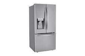
- Applications: engines, refridgerators, air-condition,... 

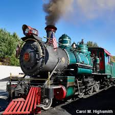
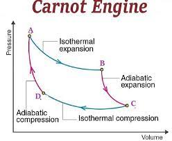
efficiency \(\leq 1-\frac{T_2}{T_1}\)

Heat engine: Carnot cycle

History

Laws of thermodynamics

Zeroth law:

Temperature can be measured. $$T_A = T_B \quad \mathrm{if} \quad A \ \mathrm{and} \ B \ \mathrm{are} \ \mathrm{in} \ \mathrm{equilibrium}.$$

First law (Claussius 1850, Helmholtz 1847):

Energy is conserved.
$${\color{aqua} d}U = {\color{orange} \delta} Q - {\color{orange} \delta} W$$ Second law (Carnot 1824, Claussius 1854, Kelvin):

Heat cannot be fully transformed into work. $${ \color{aqua} d} S \geq \frac{{\color{orange} \delta} Q}{T}$$ Third law: We cannot bring the system into the absolute zero
temperature in a finite number of steps. $$ \lim_{T \rightarrow 0} S(T) = 0$$

History

Local equilibrium thermodynamics (1st half of 20th cent.)

- Onsager, Rayleigh...

- Systems close to equilibrium - linear response theory

-  Local equilibrium: subsystems a,b,c are each in equilibrium  

Total entropy \(S \approx S^a + S^b + S^c + \dots\)

Entropy production \(\sigma^a = \frac{d S^a}{d t} = \sum_i Y_i^a J_i^a \)

\(Y_i^a\) - thermodynamic forces; \(J_i^a\) - thermodynamic currents

4th Law of thermodynamics (Onsager 1931): \( \sigma = \sum_{ij} L_{ij} \Gamma_i \Gamma_j\)

 \(\Gamma_i = Y_i^a - Y_i^b \) - afinity, \(L_{ij}\) - symmetric

History and now

Stochastic thermodynamics (90s of 20th century - present)

- Evans, Jarzynski, Crooks, Seifert, van den Broek,....

- Mesoscopic systems far from equilibrium 

- Combines stochastic calculus and non-equilibrium thermodynamics

- Main results: Trajectory thermodynamics, Fluctuation theorems, Thermodynamic uncertainty relations, Speed limit theorems,...

- Applications: colloidal particles and soft matter, biochemistry, molecular motors

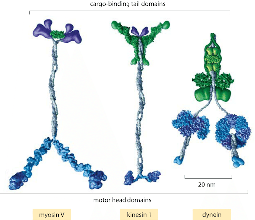
Molecular motor: myosin walking on actin filament

efficiency \(\lesssim 1\)

Main results of stochastic thermodynamics

Stochastic thermodynamics

1.) Consider linear Markov (= memoryless) with distribution \(p_i(t)\).

Its evolution is described by master equation

$$ \dot{p}_i(t) = \sum_{j} [w_{ij} p_{j}(t) - w_{ji} p_i(t) ]$$

\(w_{ij}\) is transition rate. 

2.) Entropy of the system - Shannon entropy  \(S(P) = - \sum_i p_i \log p_i\). Equilibrium distribution is obtained by maximization of \(S(P)\) under the constraint of average energy \( U(P) = \sum_i p_i \epsilon_i \)

$$ p_i^{eq} = \frac{1}{Z} \exp(- \beta \epsilon_i) \quad \mathrm{where} \ \beta=\frac{1}{k_B T}, Z = \sum_j \exp(-\beta \epsilon_j)$$

Stochastic thermodynamics

3.) Detailed balance - stationary state (\(\dot{p}_i = 0\) ) coincides with the equilibrium state (\(p_i^{eq}\)). We obtain

$$\frac{w_{ij}}{w_{ji}} = \frac{p_i^{eq}}{p_j^{eq}} = e^{\beta(\epsilon_j - \epsilon_i)}$$

4.) Second law of thermodynamics: 

$$\dot{S} = - \sum_i \dot{p}_i \log p_i = \frac{1}{2} \sum_{ij} (w_{ij} p_j - w_{ji} p_i) \log \frac{p_j}{p_i}$$

$$ =\underbrace{\frac{1}{2} \sum_{ij} (w_{ij} p_j - w_{ji} p_i) \log \frac{w_{ij} p_j}{w_{ji} p_i}}_{\dot{S}_i} + \underbrace{\frac{1}{2} \sum_{ij} (w_{ij} p_j - w_{ji} p_i) \log \frac{w_{ji}}{w_{ij}}}_{\dot{S}_e}$$

\( \dot{S}_i \geq 0 \) - entropy production rate (2nd law of TD)

\(\dot{S}_e = \beta \dot{Q}\) entropy flow rate

Stochastic thermodynamics

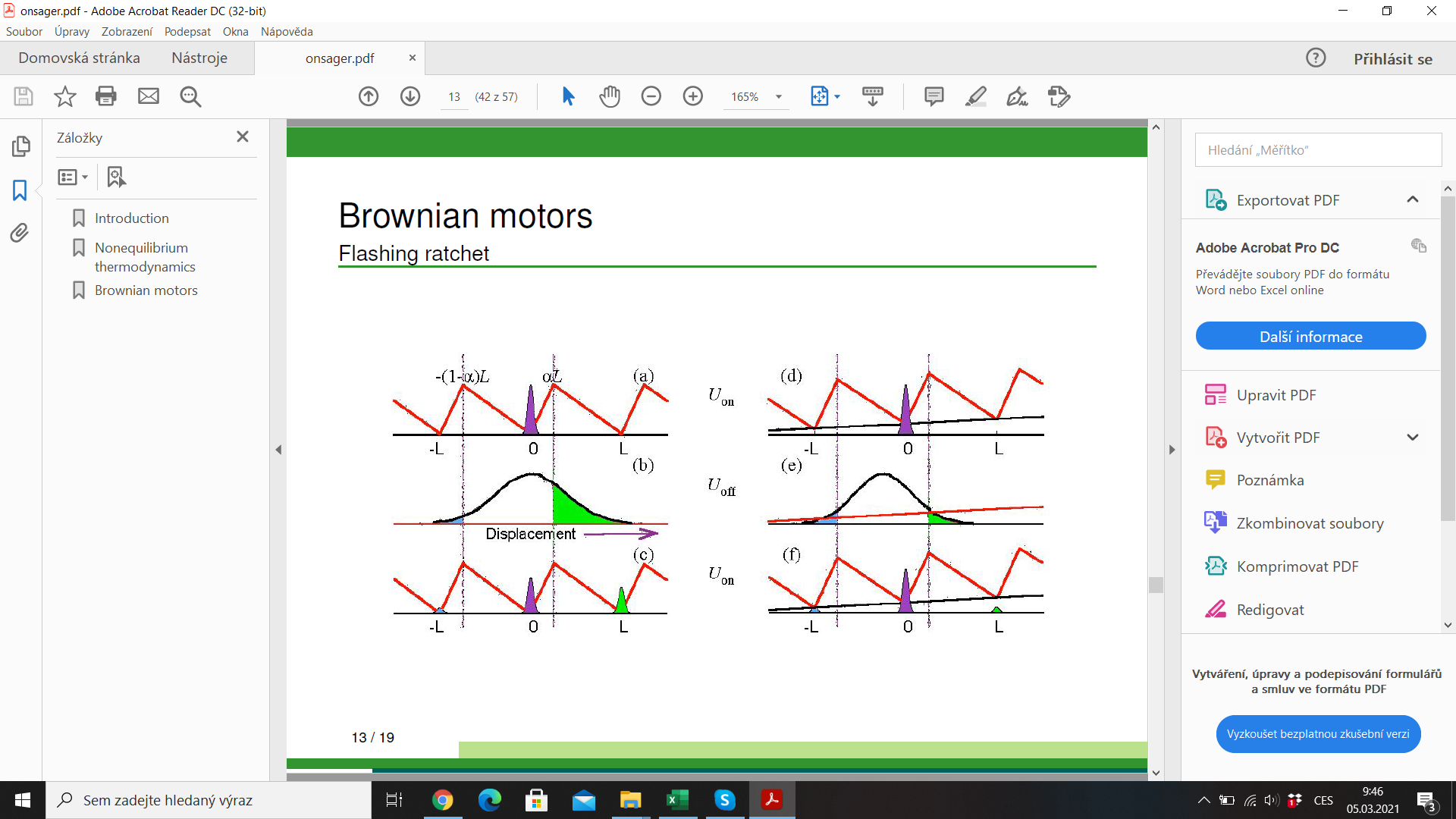
5.) Trajectory thermodynamics - consider stochastic trajectory

\(x(t)= (x_0,t_0;x_1,t_1;\dots)\). Energy \(E_x = E_x(\lambda(t))\), \(\lambda(t)\) - control protocol

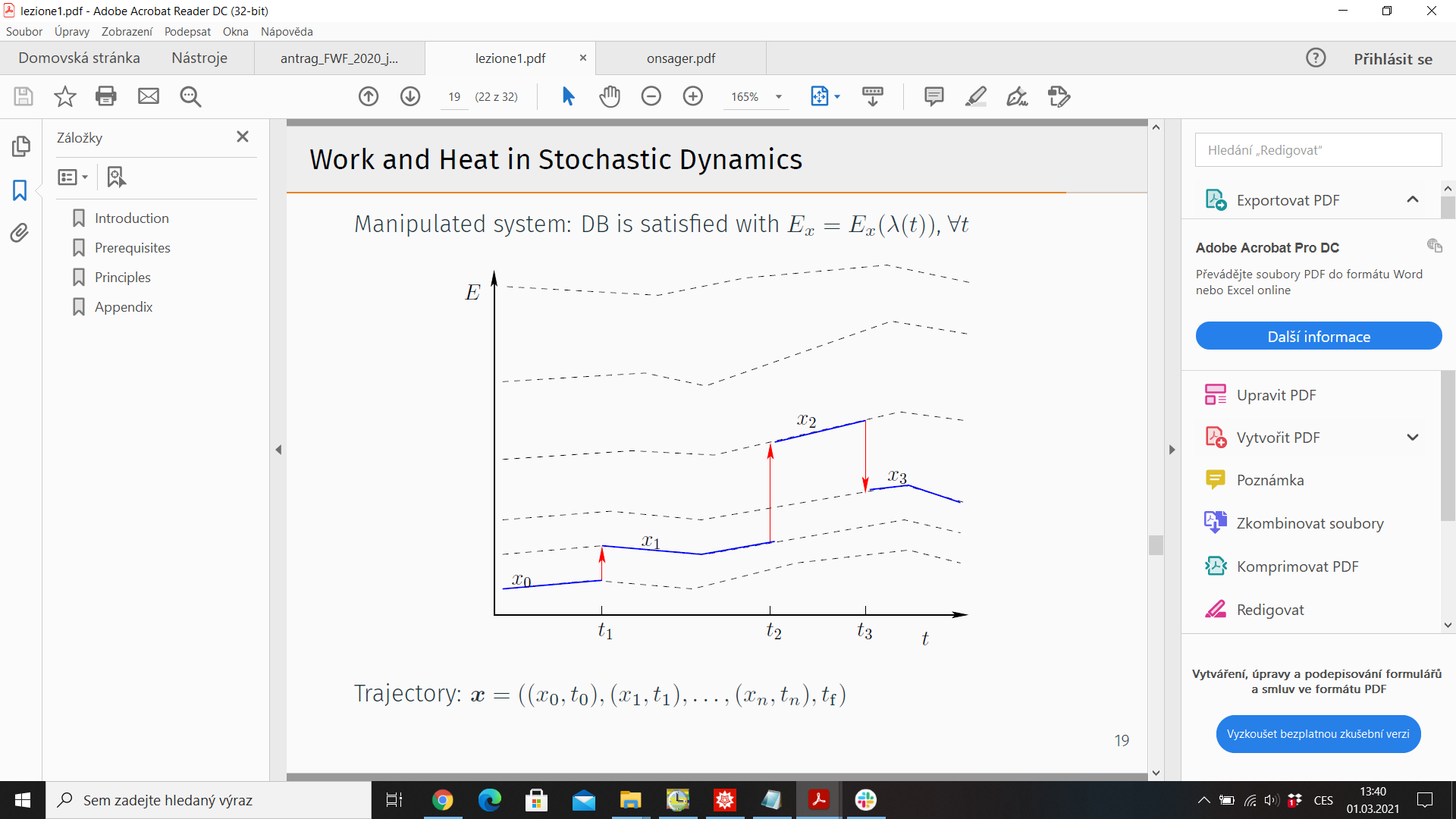
Probability of observing \( x(t)\): \(\mathcal{P}(x(t)\))

Time reversal \(\tilde{x}(t) = x(T-t)\)

Reversed protocol \(\tilde{\lambda}(t) = \lambda(T-t)\)

Probability of observing reversed trajectory under reversed protocol \(\tilde{\mathcal{P}}(\tilde{x}(t))\)

Stochastic thermodynamics

6.) Fluctuation theorems

Trajectory entropy: \(s(t) = - \log p_x(t)\)

Trajectory 2nd law \(\Delta s = \Delta s_i + \Delta s_e\)

Relation to the trajectory probabilities

$$\log \frac{\mathcal{P}(x(t))}{\tilde{\mathcal{P}}(\tilde{x}(t))} = \Delta s_i$$

Detailed fluctuation theorem

$$\frac{P(\Delta s_i)}{\tilde{P}(-\Delta s_i)} = e^{\Delta s_i}$$

Integrated fluctuation theorem $$ \langle e^{- \Delta s_i} \rangle = 1 \quad \Rightarrow \langle \Delta s_i \rangle = \Delta S_i \geq 0$$

Thermodynamics of structure-forming systems

Motivation

• Many systems form structures: molecules of atoms, clusters of colloidal particles, (bio)polymers or micelles
• We study the thermodynamics of structure-forming systems
• For small systems, we get a correction to Shannon entropy
• We apply the results to several physical systems
• We derive fluctuation theorems for structure-forming systems

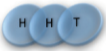
Toy model - magnetic coin model

We consider a coin with two states: head             and tail

The coins are magnetic and can stick together 

How many states we get for N coins?

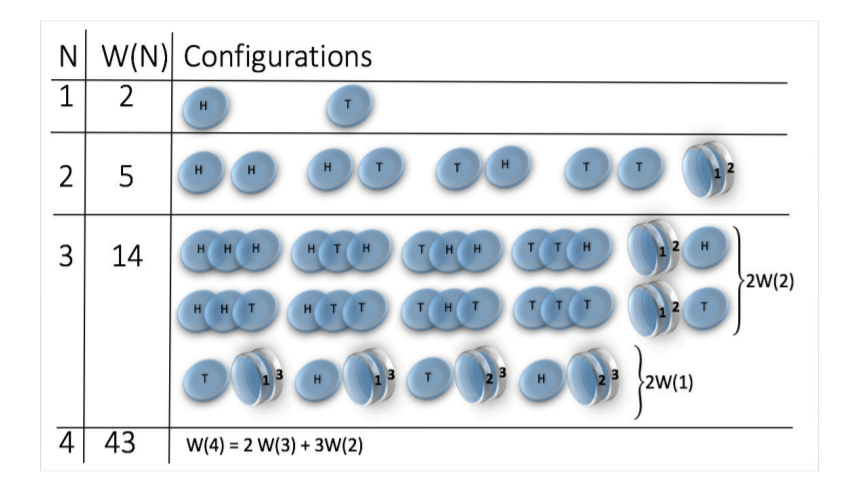
\(W(N) \sim N^N\)

(non-magnetic coins \(W(N) = 2^N\))

picture taken from: H. J. Jensen et al 2018 J. Phys. A: Math. Theor. 51 375002

Multiplicity and entropy

of structure-forming systems

Boltzmann entropy formula: \(S(n_i) = k_B \log W(n_i)\) 

where \(W\) is multiplicity

(number of microstates corresponding to a mesostate \(n_i\))

Microstate: state of each particle

       if more particles are bound to a molecule, then state of each molecule

Mesostate: how many particles and/or molecules are in given state

Example: magnetic coin model: 3 coins, magnetic

                 microstates                       mesostate                 multiplicity

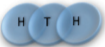
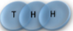
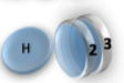
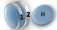
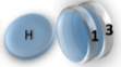
2 x           1x

1 x          1x

3

3

How to calculate a multiplicity?

1. Consider a mesostate
2. Make all permutations of particles
3. Some microstates are overrepresented - calculate how many permutations belong to the same microstate

Examples

2 x           1x

1 x          1x

1    1   2   2    3   3

2   3   1   3    1    2

3   2   3   1    2    1

1    1   2   2    3   3

2   3   1   3    1    2

3   2   3   1    2    1

= (1,2,3) , (2,1,3)

= (1,3,2) , (3,1,2)

= (2,3,1) , (3,2,1)

= (1,2,3) , (1,3,2)

= (2,1,3) , (2,3,1)

= (3,1,2) , (3,2,1)

General formula for multiplicity

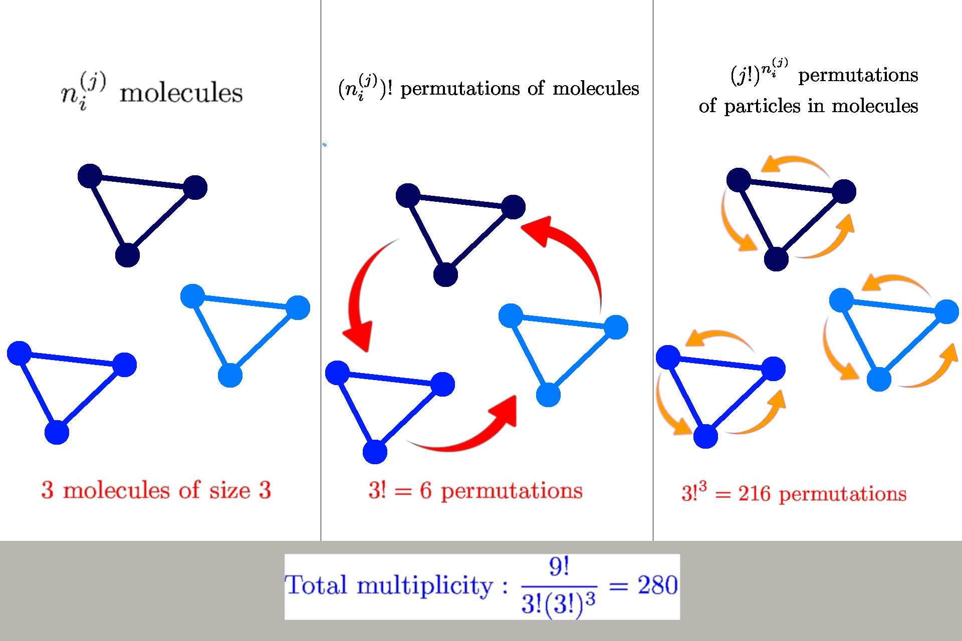
General formula: \(W(n_i^{(j)}) = \frac{n!}{\prod_{ij} n_i^{(j)}!  {\color{aqua} (j!)^{n_i^{(j)}}}}\)  

we have \(n_i^{(j)}\) molecules of size \(j\) in a state \(s_i^{(j)}\)

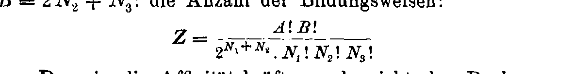
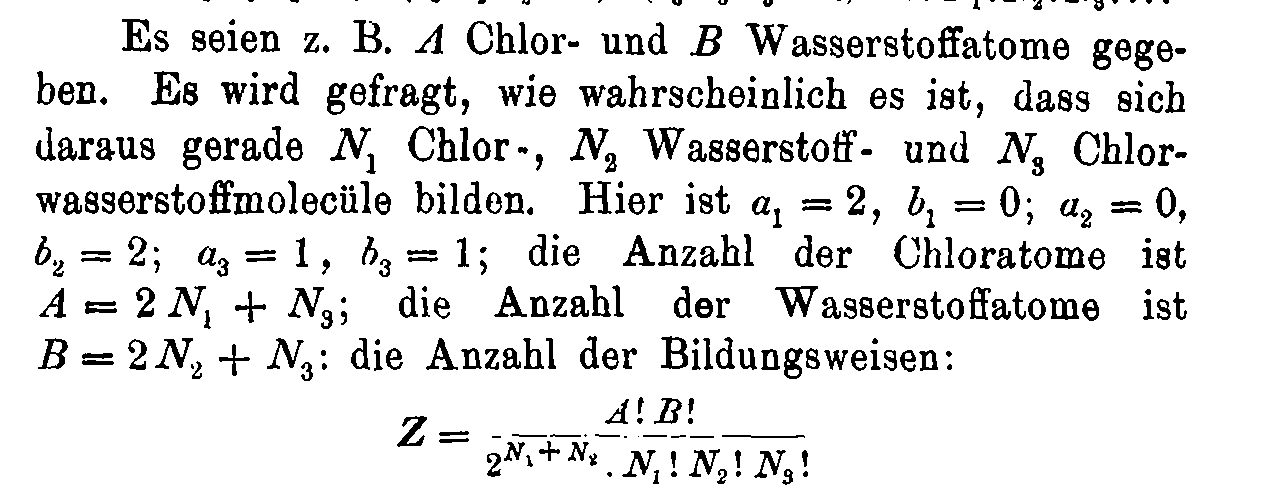
Boltzmann's 1884 paper

Entropy of structure-forming systems

$$ S =  \log W \approx n \log n - \sum_{ij} \left(n_i^{(j)} \log n_i^{(j)} - n_i^{(j)} + {\color{aqua} n_i^{(j)} \log j!}\right)$$

Introduce "probabilities" \(\wp_i^{(j)} = n_i^{(j)}/n\)

$$\mathcal{S} = S/n = - \sum_{ij} \wp_i^{(j)} (\log \wp_i^{(j)} {\color{aqua}- 1}) {\color{aqua}- \sum_{ij} \wp_i^{(j)}\log  \frac{j!}{n^{j-1}}}$$

Finite interaction range: concentration \(c = n/b\) 

$$\mathcal{S} = S/n = - \sum_{ij} \wp_i^{(j)} (\log \wp_i^{(j)} {\color{aqua}- 1}) {\color{aqua}- \sum_{ij} \wp_i^{(j)}\log  \frac{j!}{{\color{orange}c^{j-1}}}}$$

Equilibrium distribution:

$$\hat{\wp}_i^{(j)} = \frac{c^{j-1}}{j!} \exp(-\alpha j - \beta \epsilon_i^{(j)})$$

normalization by solving

\(\sum_{ij} j \wp_i^{(j)} = \sum_{ij} \frac{c^{j-1}}{(j-1)!} e^{-{\color{aqua} \alpha} j - \beta \epsilon_i^{(j)}} = 1\) for \({\color{aqua} \alpha}\)

Entropy of structure-forming systems

Main properties:

• The entropy fulfills Shannon Khinchin axioms 1,3,4 but does not fulfill axiom SK 2 (it is not maximized by uniform distribution)
• The entropy fulfills Lieb-Yngvason axioms (it is additive, and it is extensive for \(c=const\) )
• The entropy fulfills Shore-Johnson axioms 1,3,4 but does not fulfill axioms SJ 2 (permutation/coordinate invariance)
• The entropy fulfills Tempesta group-composability axiom but is not symmetric in its arguments
• The scaling exponents according to Hanel-Thurner axioms are                           \(c=0,d=1\), the same as for Shannon entropy

\( \Rightarrow\) The entropy satisfies all common axiomatic schemes but it is not symmetric in probabilities

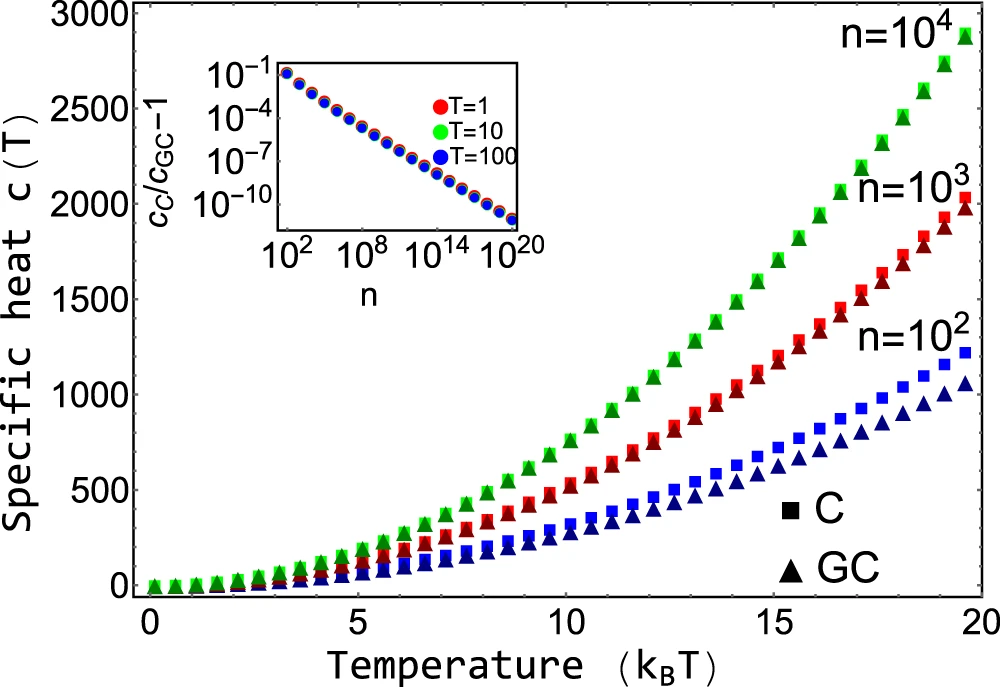
Comparison with Grand-canonical ensemble

Applications

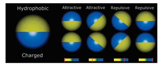
 Self-assembly of Janus particles

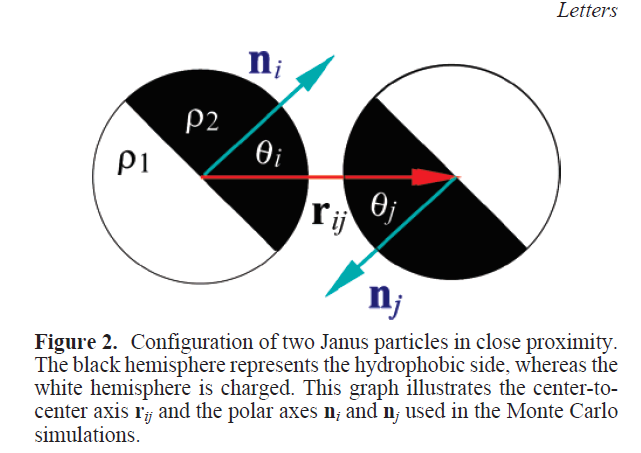
Kern-Frenkel model

Pair-wise potential: \(U^{KF}(r_{ij},n_i,n_j) = u(r_{ij}) \Omega(r_{ij},n_i,n_j) \)

Square-well interaction with hard sphere: 

$$ u(r_{ij}) = \left\{ \begin{array}{rl} \infty, & r_{ij} \leq \sigma \\  - \epsilon, & \sigma < r_{ij} < \sigma + \Delta \\ 0, & r_{ij} > \sigma + \Delta. \end{array} \right.$$

\(\Omega\) decribes orientation of particles:

Particle coverage \(\chi = \sin^2(\theta/2) = \frac{1-\cos{\theta}}{2}\)

Polymers: \(\chi = 0.3\)

Janus particles: \(\chi = 0.5\)

Crystalic structures: \(\chi = 0.6\) (stable lamellar crystals)

$$\Omega(r_{ij},n_i,n_j) = \left\{\begin{array}{rl} -1 & \mathrm{if} \  r_{ij} \cdot n_i > \cos(\theta) \ \mathrm{and} \ r_{ij} \cdot n_j > \cos(\theta)\\ 0 & \mathrm{otherwise} \end{array}  \right.$$

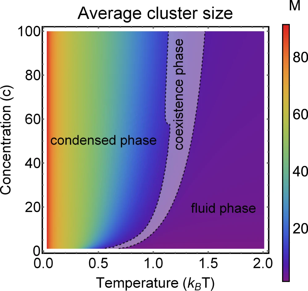
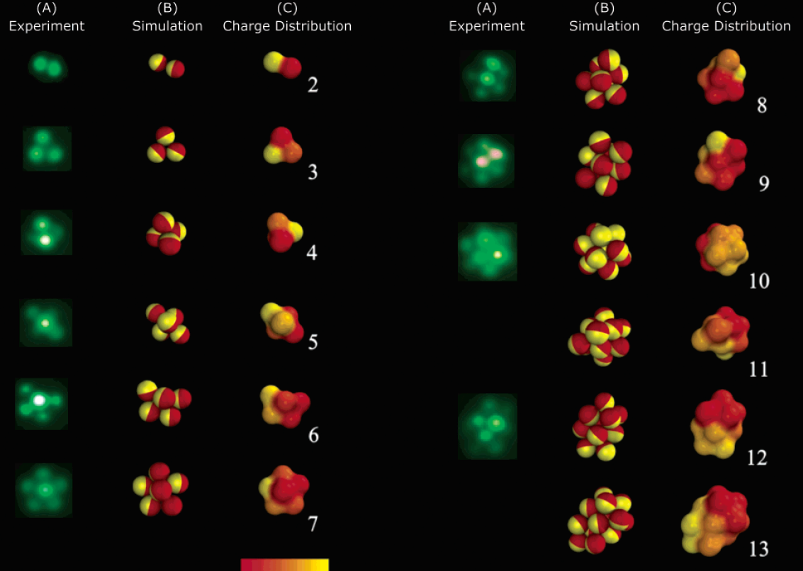
Phase diagram of Janus particles for average cluster size \(M\)

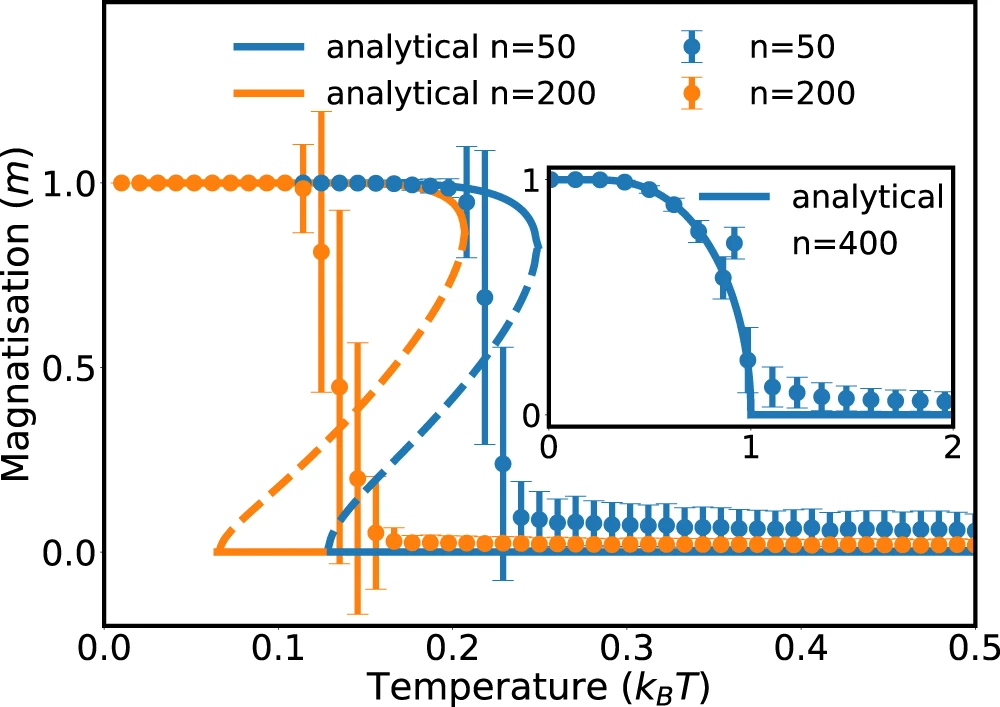
Currie-Weiss model with molecules

(= fully connected Ising model with bound states)

$$ H(\sigma_i) = - \frac{J}{n-1} \sum_{i \neq j, \ free} \sigma_i \sigma_j - h \sum_{j, \ free} \sigma_j $$

Stochastic thermodynamics of structure-forming systems

1. Linear Markov (= memoryless) with distribution \(\wp_i(t)\).

Its evolution is described by master equation

$$ \dot{\wp}_i(t) = \sum_{j} [w_{ij} \wp_{j}(t) - w_{ji} \wp_i(t) ]$$

\(w_{ij}\) is transition rate. 

2. Detailed balance

Assumptions

Stochastic thermodynamics of structure-forming systems

Results

1. Second law of thermodynamics for non-equilibrium systems

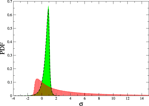
2. Detailed fluctuation theorem for structure forming systems

$$\frac{P(\Delta \sigma)}{\tilde{P}(-\Delta \sigma)} = e^{\Delta \sigma}$$

where  \(\Delta \sigma = \Delta s_i +  {\color{aqua} \log j_0 - \log j_f}\)

\(\Delta s_i\) is the trajectory entropy production

Summary

More details in: J. Korbel, S. D. Lindner, R. Hanel and S. Thurner,

Nat. Comm. 12 (2021) 1127