Overview of the main Properties of Generalized Entropies
Jan Korbel
CSH Workshop
"Holographic and other Cosmologically Relevant Entropies"
20-22 January 2025


Slides available at: https://slides.com/jankorbel
Personal web: https://jankorbel.eu
Introduction
- The main aim of the workshop is to study the relevance of entropy in cosmology
- One part of this is to focus on using generalized entropies like:
- Rényi entropy \(R_q = \frac{1}{1-q} \log \sum_i p_i^q\)
- Tsallis entropy \(S_q =\frac{1}{1-q} (\sum_i p_i^q -1) \)
- Sharma-Mittal entropy \(M_{Q,q} = \frac{1}{1-Q} ((\sum_i p_i^{q})^{\frac{1-Q}{1-q}} -1)\)
- Tsallis-Cirto entropy \(S_{q,\delta} = \sum_i p_i (\log_q 1/p_i)^\delta\)
- Kaniadakis entropy \(K_\kappa = \frac{1}{2 \kappa}\sum_i (p_i^{1+\kappa} - p_i^{1-\kappa})\)
- and other
- All these entropies are generalizations of Shannon entropy \(H = -\sum_i p_i \log p_i\)
- This talk focuses on the properties of generalized entropies
- We will go through some key aspects of entropy in thermodynamics, information theory and statistical inference
Introduction
- Generalized entropies were introduced in statistical physics to describe systems where the Boltzmann-Gibbs statistics fail
- The main applications of generalized entropies include:
- Non-extensive systems (e.g., long-range interactions)
- Non-ergodic systems (not all states are sampled equally)
- Non-exponential MaxEnt distributions
- Complex systems
- The main applications of generalized entropies include:
- Plasmas, high-energy physics, and gravitational systems
- Quantum entanglement and decoherence
- Information theory and statistical inference
- Non-physical systems, e.g., biology, linguistics, finance
Information theory:
Shannon-Khinchin axioms
with Petr Jizba (CTU in Prague)
Axiomatization from the Information theory point of view
- Continuity.—Entropy is a continuous function of the probability distribution only.
- Maximality.— Entropy is maximal for the uniform distribution.
- Expandability.— Adding an event with zero probability does not change the entropy.
- Additivity.— \(H(A \cup B) = H(A) + H(B|A)\) where \(H(B|A) = \sum_i p_i^A H(B|A=a_i)\)
-
These four axioms lead to Shannon entropy $$ H(P) = - \sum_i p_i \log p_i $$
- Many authors have considered generalizations of 4th Axiom
- We show a natural generalization covering a wide class of entropies
Shannon-Khinchin axioms
Kolmogorov-Nagumo algebra
- Let us considering a bijection \( f(x) \)
- We define addition, subtraction, multiplication, and division as follows $$x\oplus y = f(f^{-1}(x) + f^{-1}(y))$$ and similarly for other operations
- In 1930, Andrey Kolmogorov and Mitio Nagumo independently introduced a generalization called f-mean for an arbitrary continuous and injective function
$$\langle X \rangle_f := f^{-1} \left(\frac{1}{n} \sum_i f(x_i)\right)$$
- The basic property is that the mean is invariant to the transformation \(f(x) \mapsto a f(x) + b\)
- The Hölder mean is obtained for \(f(x) = x^p\)
We now replace SK4 with the following axiom:
4. Composability: Entropy of a joined system \( A \cup B\) can be expressed as \(S(A \cup B) = S(A|B) \otimes_f S(B)\), where \(S(A|B)\) is conditional entropy satisfying consistency requirements I.), II.)
I.) For independent variables \(A,B\), the joint entropy \(S(A \cup B)\) should be composable from entropies \(S(A)\) and \(S(B)\), i.e., \(S(A \cup B) = F(S(A),S(B))\)
II.) Conditional entropy should be decomposable into entropies of conditional distributions, i.e., \(S(B|A) = G\left( P_A, \{S(B|A=a_i)\}_{i=1}^m\right)\)
Kolmogorov-Nagumo algebra
P.J. & J.K. Phys. Rev. E 101, 042126
Class of admissible entropies
- Entropies fulfilling KN type of SK: $$S_q^f(P) = f\left[\left(\sum_i p_i^q\right)^{1/(1-q)}\right] = f\left[\exp_q\left( \sum_i p_i \log_q(1/p_i) \right)\right]$$
- where
- \(\exp_q(x) := \left(1 + (1-q) x\right)_+^{1/(1-q)}\)
- \(\log_q(x) := \frac{x_+^{1-q}-1}{1-q}\)
- Here \( x_+\) denotes \(\max\{x,0\}\)
- Notable examples
- \(f(x) = \log(x)\) - Rényi entropy \(R_q = \frac{1}{1-q} \log \sum_i p_i^q\)
- \(f(x) = \log_q(x)\) - Tsallis entropy \(S_q = \frac{1}{1-q}(\sum_i p_i^q -1)\)
- \(f(x) = \log_Q(x)\) - Sharma-Mittal entropy \(M_{Q,q} = \frac{1}{1-Q} ((\sum_i p_i^{q})^{\frac{1-Q}{1-q}} -1)\)
- Note that the entropy can be written as a KN mean
Statistical inference:
Shore-Johnson axioms
with Petr Jizba (CTU in Prague)
Shore-Johnson axioms
- Axiomatization from the Maximum entropy
principle point of view Principle of maximum entropy is an inference method and it should obey some statistical consistency requirements.- Shore and Johnson set the consistency requirements:
- Uniqueness.—The result should be unique.
- Permutation invariance.—The permutation of states should not matter.
- Subset independence.—It should not matter whether one treats disjoint subsets of system states in terms of separate conditional distributions or in terms of the full distribution.
- System independence.—It should not matter whether one accounts for independent constraints related to disjoint subsystems separately in terms of marginal distributions or in terms of full-system constraints and joint distribution.
- Maximality.—In absence of any prior information the uniform distribution should be the solution.
P.J. & J.K. Phys. Rev. Lett. 122 (2019), 120601
Uffink class of entropies
Entropies fulfilling SJ axioms is the same as for SK axioms: $$S_q^f(P) = f\left[\left(\sum_i p_i^q\right)^{1/(1-q)}\right] = f\left[\exp_q\left( \sum_i p_i \log_q(1/p_i) \right)\right]$$
MaxEnt distribution: q-exponential
$$p_i = \frac{1}{Z_q} \exp_q\left(-\hat{\beta} \Delta E_i \right)$$
$$ Z_q = \sum_i \left[\exp_q\left(-\hat{\beta} \Delta E_i \right)\right]$$
$$\hat{\beta} = \frac{\beta}{q f'\left(Z_q\right) Z_q}$$
Conclusions: Uffink class of entropies can be used as a measure of information as well as for Maximum entropy principle
composition rule of \(p_{ij} \propto \exp_q (-\beta (E_i + E_j)) \)
$$\frac{1}{p_{ij} Z_q(P)} = \frac{1}{u_{i} Z_q(U)} \otimes_q \frac{1}{v_{j} Z_q(V)} $$
or in terms of escort distributions \(P_{ij}(q) = p_{ij}^q/\sum_{ij} p_{ij}^q \)
$$ \frac{P_{ij}(q)}{p_{ij}} = \frac{U_{i}(q)}{u_{i}}\ + \ \frac{V_{j}(q)}{v_{j}} - 1$$
Composition rule for
q-exponentials
Calibration invariance
of MaxEnt principle
Calibration invariance
of MaxEnt principle
- The Principle of maximum entropy is used in physics and other fields, including statistical inference
- In physics, it actually consists of two parts:
- Finding a distribution (MaxEnt distribution) that maximizes entropy under given constraints
- Plugging the distribution into the entropic functional and calculating physical quantities as thermodynamic potentials, temperature, or response coefficients (specific heat, compressibility, etc.).
- Only 1.) + 2.) uniquely characterize the properties of a physical system
- When MaxEnt is only used to obtain a distribution, there can be more combinations of entropy and constraints, yielding the same distribution
J.K. Entropy 23 (2021) 96
Calibration invariance
of MaxEnt principle
- Typically, one can relate the Langrange multipliers to physical quantities
- In the case of Shannon entropy with normal constraints, Langange functional is $$L(p) = - \sum_i p_i \log p_i - \alpha (\sum_i p_i - 1) - \beta (\sum_i p_i \epsilon_i - U)$$
- \(\beta\) is the inverse temperature \(\beta= \frac{1}{k_B T}\)
- \(\alpha\) is related to free energy \(-\frac{\alpha}{\beta} = F\)
- Are these relations still conserved when the MaxEnt distribution is the same but entropy and/or constraints change?
Example: \(f(S)\)
- Maximizing entropy \(S\) leads to the same MaxEnt distribution as maximizing \(f(S)\) where \(f\) is an increasing function
- The Lagrange fuction is $$L_f = f(S) - \alpha_f (\sum_i p_i -1) \beta_f (\sum_i p_i \epsilon_i-U)$$
- By using the method of Lagrange multipliers, we get that
- \(\beta_f = f'(S) \beta\)
- \(\alpha_f = f'(S) \alpha\)
- This transformation actually forms a group:
- if \(g(x) = f_1(f_2(x))\) then \(\beta_g = f_1'(f_2(S)) f_2'(S) \beta\)
- Examples:
- Rényi and Tsallis entropy \(R_q = \frac{1}{1-q} \ln[1+(1-q)S_q]\)
- Shannon entropy and entropy power \(P(p) = \prod_i (1/p_i)^{p_i}\) the relation is \(P = \exp(H)\)
Thermodynamics of exponential KN averages
with Fernando Rosas (ICL London) and Pablo Morales (Araya, Japan)
Kolmogorov-Nagumo averages revisited
- The arithmetic mean can be uniquely determined from the class of KN-means by the following two properties:
- Homogeneity \(\langle a X \rangle = a \langle X \rangle \)
- Translation invariance \( \langle X +c \rangle = \langle X \rangle +c\)
- Note that the Hölder means (\(f(x)=x^p\)) satisfy Property 1 but not property 2
- What is the class of means that satisfies Property 2?
Exponential KN averages
- The solution is given by the function \(f(x) = (e^{\gamma x}-1)/\gamma\) and the inverse function is \(f^{-1}(x) = \frac{1}{\gamma} \ln (1+\gamma x)\)
- This leads to the exponential KN mean$$ \langle X \rangle_\gamma = \frac{1}{\gamma} \ln \left(\sum_i \exp(\gamma x_i)\right) $$
- We recover the arithmetic mean by \(\gamma \rightarrow 0\)
- Note that one can relate \(q\) and \(\gamma\) as \(\gamma = 1-q\)
- Property 2 is important for thermodynamics since the average energy \(\langle E \rangle\) does not depend on the energy of the ground state
- The additivity is preserved for independent variables
$$\langle X + Y \rangle_\gamma = \langle X \rangle_\gamma + \langle Y \rangle_\gamma \Leftrightarrow X \perp \!\!\! \perp Y$$
- The general additivity formula is given as $$ \langle X + Y \rangle_\gamma = \langle X + \langle Y|X \rangle_\gamma\rangle_\gamma$$ where the conditional mean is given as $$ \langle X | Y \rangle_\gamma = \frac{1}{\gamma} \ln \left(\sum_i p_i \exp(\gamma \langle Y|X = x_i\rangle_\gamma ) \right) $$
- The exponential KN mean is closely related to the cumulant generating function $$M_\gamma(X) = \ln \langle \exp(\gamma X)\rangle = \gamma \langle X \rangle_\gamma $$
Exponential KN averages
Rényi entropy as exponential KN average
- Rényi entropy can be naturally obtained as the exponential KN average of the Hartley information \(\ln 1/p_k\)
- We define the Rényi entropy as $$ R_\gamma(P) = \frac{1}{1-\gamma} \langle \ln 1/p_k \rangle_\gamma = \frac{1}{\gamma(1-\gamma)} \ln \sum_k p_k^{1-\gamma}$$
- The role of the prefactor will be clear later, but one of the reasons is that the limit \(\gamma \rightarrow 1\) is the well-defined Burg entropy \(- \sum_k \ln p_k\)
- We also naturally obtain the conditional entropy $$ R_\gamma(X,Y) = R_\gamma(X) + R_\gamma(Y|X)$$
P.M., J.K. & F. E. R. New J. Phys 25 (2023) 073011
Equilibrium thermodynamics of Exponential KN Averages
- Let us now consider thermodynamics, where all quantities are exponential KN averages
- We consider that the system entropy is described by Rényi entropy
- The internal energy is described as the KN average of the energy spectrum \(\epsilon\) $$U_\gamma^\beta := \frac{1}{\beta} \langle \beta \epsilon \rangle_\gamma = \frac{1}{\beta \gamma} \ln \sum_i p_i \exp(\beta \gamma \epsilon_i)$$
- The inverse temperature \(\beta = \frac{1}{k_B T}\) ensures that the energy has correct units
MaxEnt distribution
- Let us now calculate the MaxEnt distribution obtained from Rényi entropy with given internal energy \(U^\beta_\gamma \)
- The Lagrange function is $$ \mathcal{L} = R_\gamma - \alpha_0 \sum_i p_i - \alpha_1 \frac{1}{\beta}\langle \beta \epsilon \rangle_\gamma$$
- The MaxEnt distribution \(\pi_i\) can be obtained from
$$ \frac{1}{\gamma} \frac{\pi_i^{-\gamma}}{\sum_k \pi_k^{1-\gamma}} - \alpha_0 - \frac{\alpha_1}{\beta \gamma} \frac{e^{\gamma \beta \epsilon_i}}{\sum_k \pi_k e^{\gamma \beta \epsilon_k}} = 0$$
- By multiplying by \(\pi_i\) and summing over \(i\) we obtain \(\alpha_0 = \frac{1-\alpha_1}{\gamma}\) and therefore $$\pi_i = \frac{\left(\sum_k \pi_k e^{\gamma \beta \epsilon_k}\right)^{1/\gamma}}{\left(\sum_k \pi_k^{1-\gamma}\right)^{1/\gamma}} \exp(-\beta \epsilon_i) = \frac{\exp(-\beta \epsilon_i)}{Z^\beta}$$
MaxEnt distribution
- We obtained Boltzmann distribution from non-Shannonian entropy with non-arithmetic constraint
- We immediately obtain that $$\ln \pi_i = - \beta(\epsilon_i - U_\gamma^\beta(\pi)) - (1-\gamma) R_\gamma(\pi)$$ which leads to $$\ln \sum_k e^{-\beta \epsilon_k} = (1-\gamma) R_\gamma - \beta U^\beta_\gamma = \Psi_\gamma - \gamma R_\gamma$$ where \(\Psi_\gamma = R_\gamma - \beta U_\gamma^\beta\) is the Massieu function
- The Helmholtz free energy can be expressed as $$F^\beta_\gamma(\pi) = U_\gamma^\beta(\pi)- \frac{1}{\beta} R_\gamma(\pi) = \frac{1}{(\gamma-1) \beta} \ln \sum_k e^{(\gamma-1)\beta \epsilon_k}.$$
- Thus, although we get the same distribution as for the ordinary thermodynamics, the thermodynamic relations are different!
Thermodynamic interpretation
- We calculate equilibrium Rényi entropy $$ \mathcal{R}_\gamma^\beta = \frac{1}{\gamma(1-\gamma)} \ln \sum_i \left(\frac{e^{-\beta \epsilon_i}}{Z^\beta}\right)^{1-\gamma} = \frac{1}{\gamma(1-\gamma)} \ln \sum_i e^{-(1-\gamma)\beta} - \frac{1}{\gamma} \ln Z^\beta $$
- Thus we get that Rényi entropy of a Boltzmann distribution is $$\mathcal{R}_\gamma^\beta = -\frac{\beta}{\gamma} \left(\mathcal{F}^{(1-\gamma) \beta} - \mathcal{F}^{\beta}\right)$$
- By defining \(\beta' = (1-\gamma)\beta \quad \Rightarrow \quad \gamma = 1-\frac{\beta'}{\beta}\) we can express it as
$$ \mathcal{R}_\gamma^\beta = \beta^2 \, \frac{\mathcal{F}^{\beta'} - \mathcal{F}^\beta}{\beta'-\beta} $$
which is the \(\beta\) rescaling of the free energy difference.
- This can be interpreted as the maximum amount of work the system can perform by quenching the system from inverse temperature \(\beta\) to inverse temperature \(\beta'\).
- This has been first discovered by John Baez.
- By taking \(\gamma \rightarrow 0\) we recover the relation between entropy and free energy $$\mathcal{S}^\beta = \beta^2 \left(\frac{\partial \mathcal{F}^\beta}{\partial \beta}\right)$$
- As shown before, the free energy can be expressed as $$ \mathcal{F}_\gamma^\beta = \mathcal{F}^{(1-\gamma)\beta}$$ so it is clear that the temperature is rescaled from \(\beta\) to \((1-\gamma)\beta\)
- Finally the internal energy can be expressed as $$ \mathcal{U}^\beta_\gamma = \frac{\beta' \mathcal{F}^{\beta'} - \beta \mathcal{F}^\beta}{\beta'-\beta} = - \frac{\Psi^{\beta'}-\Psi^\beta}{\beta'-\beta}$$
- Again, by taking \(\gamma \rightarrow 0\) we recover
$$ \mathcal{U}^\beta = - \left(\frac{\partial \Psi^\beta}{\partial \beta}\right)\, $$
Thermodynamic interpretation
Asymptotic scaling:
scaling expansion
with Rudolf Hanel and Stefan Thurner (both CSH)
Classification of statistical complex systems
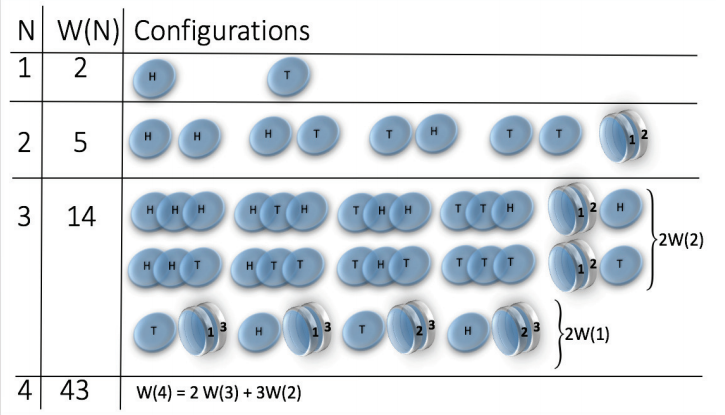
- Many examples of complex systems are statistical systems
- Statistical systems near the thermodynamic limit \(N \rightarrow \infty \) can be characterized by asymptotics of its sample space \(W(N)\) - space of all possible configurations
-
Asymptotic behavior can be described by scaling expansion
- Coefficients of scaling expansion correspond to scaling exponents
- Scaling exponents completely determine universality classes
- We can find corresponding extensive entropy
- generalization of (c,d)-entropy \(^\star\)
\(^\star\) R.H., S.T. EPL 93 (2011) 20006
Rescaling the sample space
- How does the sample space change when we rescale its size \( N \mapsto \lambda N \)?
- The ratio behaves like \(\frac{W(\lambda N)}{W(N)} \sim \lambda^{c_0} \) for \(N \rightarrow \infty\)
- the exponent \(c_0\) can be extracted by \(\frac{d}{d\lambda}|_{\lambda=1}\): \(c_0 = \lim_{N \rightarrow \infty} \frac{N W'(N)}{W(N)}\)
- For the leading term we have \(W(N) \sim N^{c_0}\).
- Is it only possible scaling? We have \( \frac{W(\lambda N)}{W(N)} \frac{N^{c_0}}{(\lambda N)^{c_0}} \sim 1 \)
- Let us use the other rescaling \( N \mapsto N^\lambda \)
- The we get that \(\frac{W(N^\lambda)}{W(N)} \frac{N^{c_0}}{N^{\lambda c_0}} \sim \lambda^{c_1}\)
- First correction is \(W(N) \sim N^{c_0} (\log N)^{c_1}\)
- It is the same scaling like for \((c,d)\)-entropy
-
Can we go further?
-
We define the set of rescalings \(r_\lambda^{(n)}(x) := \exp^{(n)}(\lambda \log^{(n)}(x) \) )
- \( f^{(n)}(x) = \underbrace{f(f(\dots(f(x))\dots))}_{n \ times}\)
- \(r_\lambda^{(0)}(x) = \lambda x\), \(r_\lambda^{(1)}(x) = x^\lambda\), \(r_\lambda^{(2)}(x) = e^{\log(x)^\lambda} \), \(r_\lambda^{(-1)}(x) = x + \log \lambda\)
- They form a group: \(r_\lambda^{(n)} \left(r_{\lambda'}^{(n)}\right) = r_{\lambda \lambda'}^{(n)} \), \( \left(r_\lambda^{(n)}\right)^{-1} = r_{1/\lambda}^{(n)} \), \(r_1^{(n)}(x) = x\)
-
We repeat the procedure: \(\frac{W(N^\lambda)}{W(N)} \frac{N^{c_0} (\log N)^{c_1} }{N^{\lambda c_0} (\log N^\lambda)^{c_1}} \sim 1\),
- We take \(N \mapsto r_\lambda^{(2)}(N)\)
- \(\frac{W(r_\lambda^{(2)}(N))}{W(N)} \frac{N^{c_0} (\log N)^{c_1} }{r_\lambda^{(2)}(N)^{c_0} (\log r_\lambda^{(2)}(N))^{c_1}} \sim \lambda^{c_2}\),
- Second correction is \(W(N) \sim N^{c_0} (\log N)^{c_1} (\log \log N)^{c_2}\)
Rescaling the sample space
- General correction is given by \( \frac{W(r_\lambda^{(k)}(N))}{W(N)} \prod_{j=0}^{k-1} \left(\frac{\log^{(j)} N}{\log^{(j)}(r_\lambda^{(k)}(N))}\right)^{c_j} \sim \lambda^{\bf c_k}\)
-
Possible issue: what if \(c_0 = +\infty\)?
-
Then \(W(N)\) grows faster than any \(N^\alpha\)
- We replace \(W(N) \mapsto \log W(N)\)
- The leading order scaling is \(\frac{\log W(\lambda N)}{\log W(N)} \sim \lambda^{c_0} \) for \(N \rightarrow \infty\)
- So we have \(W(N) \sim \exp(N^{c_0})\)
-
Then \(W(N)\) grows faster than any \(N^\alpha\)
- If this is not enough, we replace \(W(N) \mapsto \log^{(l)} W(N)\) so that we get finite \(c_0\)
- General expansion of \(W(N)\) is $$W(N) \sim \exp^{(l)} \left(N^{c_0}(\log N)^{c_1} (\log \log N)^{c_2} \dots\right) $$
J.K., R.H., S.T. New J. Phys. 20 (2018) 093007
Rescaling the sample space
$$W^{(l)}(N) \equiv \log^{(l+1)}(W(x)) = \sum_{j=0}^n c_j^{(l)} \log^{(j+1)}(N) + \mathcal{O} (\phi_n (N))$$
Scaling Expansion
- Previous formula can be expressed in terms of Poincaré asymptotic expansion
- Coefficients of the expansion are scaling exponents and can be calculated from:
$$ c^{(l)}_k = \lim_{N \rightarrow \infty} \log^{(k)}(N) \left( \log^{(k-1)} \left(\dots\left( \log N \left(\frac{N W'(N)}{\prod_{i=0}^l \log^{(i)}(W(N))}-c^{(l)}_0\right)-c^{(l)}_1\right) \dots\right) - c^{(l)}_k\right)$$
Extensive entropy
- We can do the same procedure with entropy \(S(W)\)
- Leading order scaling: \( \frac{S(\lambda W)}{S(W)} \sim \lambda^{d_0}\)
- First correction \( \frac{S(W^\lambda)}{S(W)} \frac{W^{d_0}}{W^{\lambda d_0}} \sim \lambda^{d_1}\)
- First two scalings correspond to \((c,d)\)-entropy for \(c= 1-d_0\) and \(d = d_1\)
- Scaling expansion of entropy $$S(W) \sim W^{d_0} (\log W)^{d_1} (\log \log W)^{d_2} \dots $$
-
Requirement of extensivity \(S(W(N)) \sim N\) determines the relation between \(c\) and \(d\) :
- \(d_l = 1/c_0\), \(d_{l+k} = - c_k/c_0\) for \(k = 1,2,\dots\)
| Process | S(W) | |||
|---|---|---|---|---|
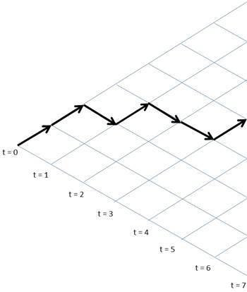
| Random walk |
0 |
1 |
0 |
|
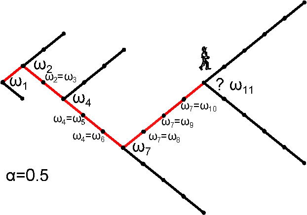
| Aging random walk |
0 |
2 |
0 |
|
| Magnetic coins * |
0 |
1 |
-1 |
|
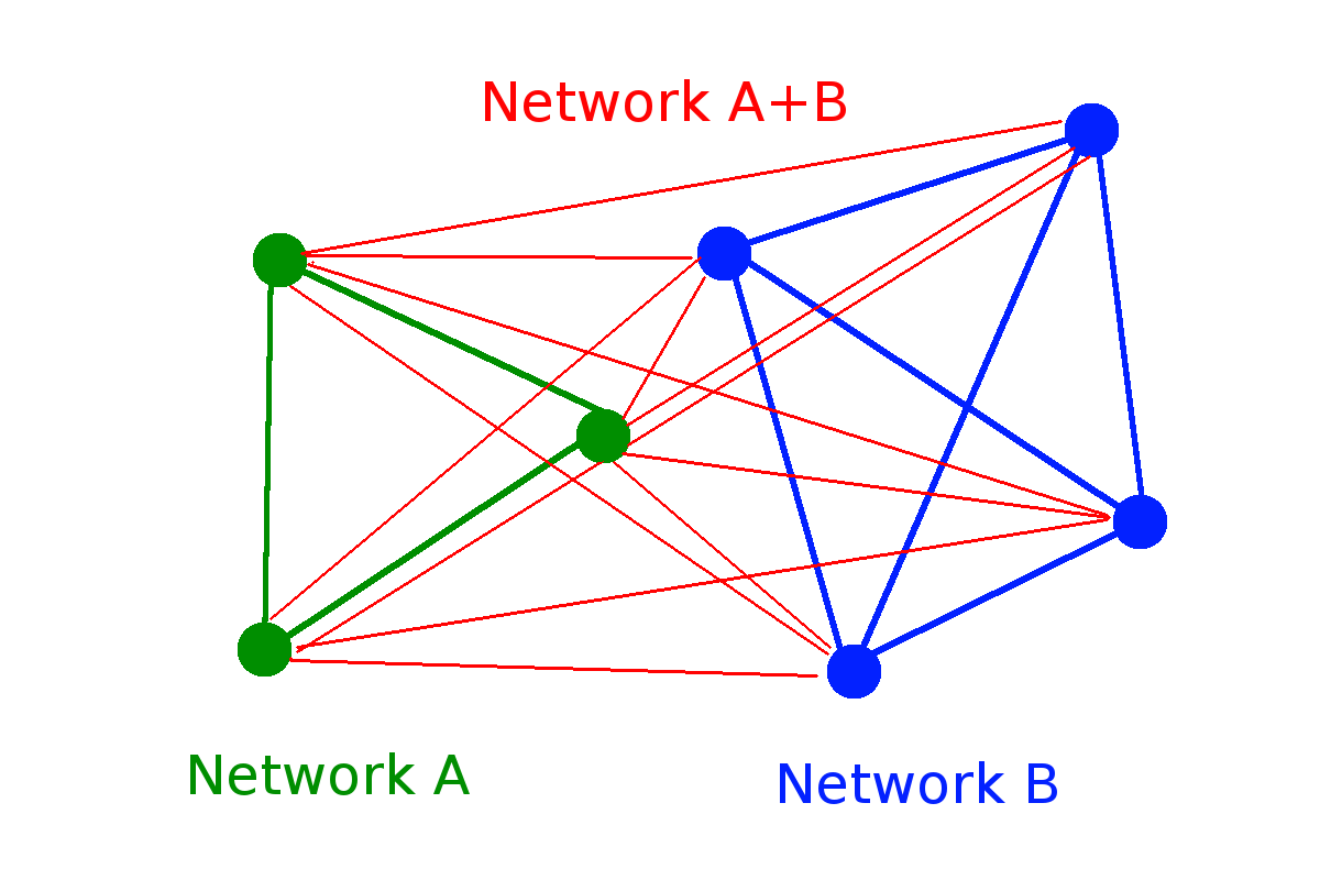
| Random network |
0 |
1/2 |
0 |
|
| Random walk cascade |
0 |
0 |
1 |
\( \log W\)
\( (\log W)^2\)
\( (\log W)^{1/2}\)
\( \log \log W\)
\(d_0\)
\(d_1\)
\(d_2\)
\( \log W/\log \log W\)
* H. Jensen et al. J. Phys. A: Math. Theor. 51 375002
\( W(N) = 2^N\)
\(W(N) \approx 2^{\sqrt{N}/2} \sim 2^{N^{1/2}}\)
\( W(N) \approx N^{N/2} e^{2 \sqrt{N}} \sim e^{N \log N}\)
\(W(N) = 2^{\binom{N}{2}} \sim 2^{N^2}\)
\(W(N) = 2^{2^N}-1 \sim 2^{2^N}\)

Parameter space of \( (c,d) \) - entropy
How does it change for one more scaling exponent?
R.H., S.T. EPL 93 (2011) 20006
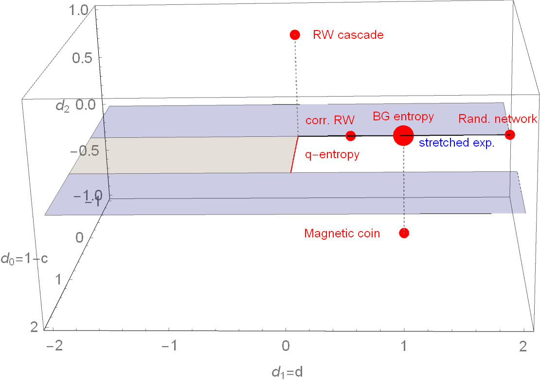
Parameter space of \( (d_0,d_1,d_2) \)-entropy
To fulfill SK axiom 2 (maximality): \(d_l > 0\), to fulfill SK axiom 3 (expandability): \(d_0 < 1\)
Interesting recent papers


1.)


2.)


3.)
