Introduction to
Statistics
Agenda
- Administrative information
- Why statistics?
- What is statistics?
- Statistical Terminology
- Types of Variables
- Relationships and Hypothesis testing
- Sampling
- Maths and statistical notation
- Descriptive statistics
- Frequency distributions
- Measures of central tendency
- Measures of dispersion
Administrative information
-
The course will be taught in 4-hours session, for four Saturdays since 25/1.
- Each session consists in 2 hours of lecture and 2 hours of seminars (flexible)
- Three different rooms:
- 25/1 - Malet Street Building Room 457
- 1/2 - Malet Street Building Room 536
- 8/2 & 15/2 Malet Street Building 422
Readings
- Agresti, Alan, and Barbara Finlay. 2009. Statistical Methods for the Social Sciences. New Jersey: Pearson Education. International edition, 4th (or 3rd) ed.
- Kellstedt, Paul M., and Guy D. Whitten. 2013. The Fundamentals of Political Science Research. Cambridge: Cambridge University Press.
-
Acock, Alan C. 2010. A Gentle Introduction to Stata. College Station, Texas: Stata Press. 3rd ed.
Readings
- People might be afraid of mathematical notations, and the readings can be a bit heavy on those. Hence, don't focus on the equations!
- It's ok if you don't understand the readings the first time. It's not ok if you continue not understanding after you finished this course, at least in part.
- If you don't have time for all of them, prioritise Agresti & Finlay or Kelstedt & Whitten
practical seminars
- We will use Stata, mainly for pedagogical reasons. If someone is interested in other packages (e.g. R), please let me know, so I can give you some guidance.
- The datasets are hosted in...
- We will try to cover a lot of ground in four weeks, so it's extremely important to practice on your own.
- Don't be afraid of Stata! It doesn't bite! It can a be a bit complicated at the beginning, just like some people ;)
Why Statistics?
- It's one of the most widely used methods for analysing (quantitative) data
- It will be useful if you are planning to use statistics for your own research.
- If you are not planning to use stats, you will most certainly find yourself reading papers using stats, and you need to understand and evaluate what are they doing
- It's fun! (Not joking). But requires some hard work.
Why statistics?
- Some people are afraid of learning stats, but you shouldn't. This is just like learning a new language, but sometimes even simpler.
- Don't focus on the equations. My job is to help you navigate though them.
- I can't do the job for you. I'm here to facilitate your own learning process, not to learn for you. It doesn't matter how many hours I stand in front of the room, you need to read, work and ask questions (!)
Why statistics?
- Do I need Maths?
- Some
- If you feel unsure, visit this website (particularly sections 1-4)
- As with everything related to maths, repetition is key.
what is statistics?
- Design
- How do we collect data?
- Description
- Describing the data
- Summarising the data
- Inference
- Making predictions to a wider population or the future
statistical terminology
The entire possible set of elements we wish study. That can be people, states, organisations, regions, etc.
The subset of elements we actually study
statistical terminology
A numerical summary of the population
A numerical summary of our sample
This summary usually contains two buts of information:
- Measures of central tendency
- Measures of variability
statistical terminology
Variable:
Anything we can measure about the subjects on our sample
Variables vary (d'oh!). That can be across the sample, and/or across time.
Statistical terminology
- The variable to be explained, described, understood.
- Is often referred as the outcome variable, and denoted with the letter Y
- It should be dependent upon something, but must not affect the independent variables
- If the dependent variable does not vary (i.e. remains constant), then we cannot explain the effect of other variables on it
statistical terminology
- Should be independent from the dependent variable, but not necessarily from other independent variables
- Presumed as the determinant of an effect or an outcome
- Usually denoted as X, explanatory or predictor variable
Types of variables
- Quantitative variables occur naturally in a numerical way
- We usualy look it in terms of ranges from low to high, which also correspond to high and low values in reality
- e.g. age, income, years of education, GDP, etc.
- Categorical variables might be expressed in numbers, but they do not mean any quantities, just codes
- e.g. gender, colours, marital status, etc.
Types of variables
- Discrete variables are much like categorical variables
- They are usually counts, which can be expressed in integer numbers (e.g. number of conflicts, count of people in a meeting, etc.)
- Continuous variables have a theoretical infinite number of outcomes(e.g. height and weight)
Types of variables
- Values that communicate differences between subjects on the characteristic being measured
-
They refer to discrete set of categories to distinguish units of analysis --> categorical variables.
- e.g. race, gender, parti affiliation
- The labels need to be exclusive.
- When they are dichotomous, they are often called dummy or binary variables.
Types of variables
- They communicate relative differences between subjects, in an ordered way (e.g. more or less). Usually related to qualities
- The values do not occur naturally, and they do not reflect quantity
- Examples:
- Educational level (not years)
- Strongly agree - Agree - Neither Agree nor Disagree - Disagree - Strongly Disagree
types of variables
- Given values that communicate exact differences between subjects on the measured characteristic
- The intervals between categories have exact meaning
- Can determine how much smaller or larger the difference is between units
- Are usually in a naturally occurring scale of some kind
- The range of values is usually fairly large (age in years, feeling thermometers, etc.)
types of variables
-
Similar to interval, but the zero in ratio variables actually denotes the absence of some quality
- E.g. Zero degrees Celsius does not mean there is no air temperature, it just denotes a different level of warmness or coolness. However, temperature expressed in Kelvin is a ratio scale because zero denotes the absence of any thermal movement
-
Ratio variables and interval variables are typically collapsed into the term “continuous” variables, and sometimes both are called interval-level
A quick note on levels of measurement
Relationships and Hypothesis Testing
Hypotheses
Null and research hypothesis
Research hypothesis
The statement of relationship or difference that the researcher is interested on. They are usually called "alternative hypotheses" and denoted H1, H2, etc.
If the null hypothesis can be rejected, we can claim that the research hypothesis is supported.
Sampling
There are several ways in which we can sample:
- stratified
- simple random
- multistage
- snowballing
random sampling
By simple random we mean that every subject in the population has the same probability of being selected for the sample.
First, we need to establish a sampling frame: the overall population from which we will draw our sample.
Random sample is usually conducted using computer programs.
bias vs random error
Random sample assumes that the error will also be random. Hence, we can estimate it with a certain level of certainty given the sample size and variation. In this way, we can now how accurate are our estimates about the general population.
Bias refers to systematic differences between the population parameters and our estimates. This can be minimised with random sampling, but is not always eliminated.
Math refresher
math refresher

statistical notation
Like learning a language, signs have meanings:
± means add and subtract
√ square root
≤ less than or equal to
≥ more than or equal to
n usually refers to sample size. Capital N is usually reserved for population size
∑ (sigma) to sum everything that comes after it
Π (pi) to multiply what comes after it
statistical notation
x is the independent variable
y is the dependent variable
x1 is the symbol for a particular observation in the independent variable
Descriptive statistics?
Univariate
- Analysis of only one variable on some characteristic
- Frequency distributions – essentially a count or distribution of values on some single variable
-
Other descriptive statistics – some summary measure that describes the data in a way not obvious by looking at the frequency distribution
descriptive statistics?
Bivariate
-
Analysis of two variables – can be simple scatter plots or histograms
Multivariate
-
Analysis of three or more variables
descriptive statistics
They are not used to draw inferences, and their analytical power is low.
They are a good starting point when we first look at the data, and can complement inferential analysis in our research.
"It does what it says on the tin" i.e. it describes the data.
Frequency Distributions

frequency distributions
Sometimes, displaying data graphically is not very useful. Why?

Frequency distributions

measures of central tendency and dispersion
central tendency
Central tendency tells us the "typical" observation in our sample. It tells us where our data is centred or clustered.
They can be helpful to get comparisons between groups, and to understand what is "normal" or "expectable" from our sample.
central tendency
Each level of data requires a different measure of central tendency
Nominal: Mode
The most common observation
Ordinal: Median
The middle observation when the data is placed in numerical order
Interval: Mean
The average across observations
central tendency: nominal
To find the central tendency of nominal data we look for the modal category
It doesn’t make sense to look for the mean w/ nominal data. If in the IQ example there were 10 observations, 3 males, coded 1, and 7 females, coded 2, the mean is 1.7, which means nothing other than there were more females in the study.
We know that there are more females in the study more easily by finding the mode; requires no calculation
central tendency: nominal
Let’s consider the following example from a larger sample dataset containing information about nurses. Suppose we want to know the typical gender of nurses. We can easily look for the modal category by running a frequency distribution.
.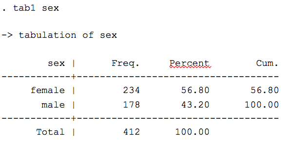
central tendency: nominal
central tendency: ordinal
The mode becomes less helpful when looking at ordinal data
It can still provide us with information, but since the categories are ranked, or ordered, we can learn more with the median. The median divides the data in half; half the observations are above the median, half are below.
The median requires the data to be ordered from lowest to highest by the variable of interest.
central tendency: ordinal
The median can be calculated through this formula:

If our dataset contains 15 observations, we add 1 and divide by 2 or (16/2 = 8) --> The 8th observation is the median
If our dataset contains 10 observations (an even number), we add 1 and divide by 2 or (11/2 = 5.5)
We look at observations 5 and 6 and find the average of those two numbers
central tendency: interval
The most common measure of central tendency is the mean, or average. We use it for interval, or continuous-level, data
The sum of all the values divided by the number of observations

central tendency: interval
measures of dispersion
Measures of dispersion (variability) measure the opposite of central tendency. They look for how spread out the data is, how much it varies.
Again, we use different measures of dispersion for different levels of measurement.
-
Nominal: categorical percentages
-
Ordinal: range and inter-quartile range
-
Interval: standard deviation and variance
dispersion: nominal
We look at the modal category (and the other categories) to see what proportion or percentage of the scores fall in that category
In the foreign aid spending example from earlier the dispersion was
-
Too much: 35%
-
About right: 45%
-
Too little: 20%
What would the percentages be if we had perfect dispersion across the categories?
What would the percentages be if we had no dispersion at all?
dispersion: nominal
There is no absolute value that we are looking for: values can range from perfectly dispersed – the same percent of observations in each category, to no dispersion – all the observations in one category.
dispersion: ordinal
When we look at ordered categories, we are interested in measures of the range. Range is the lowest observation subtracted from the observation with the highest value
If we use the previous example of exam scores:
-
54, 67, 71, 62, 50, 59, 73, 60, 64, 57
-
The range would be: 73 – 50 = 23
Therefore, the range depends upon the units in which the variables are measured.
Again, no absolute value that indicates a wide or narrow range, it's all in relative terms.
dispersion: ordinal

- The interquartile range eliminates the upper and lower 25% of observations.
- We are left with the middle 50% (line in box is median; 50th percentile
-
Eliminates outliers in skewed distributions
dispersion: interval
standard deviation
-
Standard deviation tells us how much any observation is likely to deviate from the mean
-
Or, on average, how much does an observation differ from the average
-
Dependent upon the scale in which the variable is measured
- Smaller numbers indicate less average deviation from the average
- Larger numbers indicate more average deviation from the average
Standard deviation formula

In words: The square root of the sum of each observation of x minus the mean of x, squared, and divided by n minus 1.
We can work this out by hand for small samples; but for large samples, Stata easily does this for us.
You may see this in slightly different forms depending upon the source.
Calculating standard deviation step by step
1. Calculate mean
2. Subtract mean from each observation
3. Square each residual
4. Sum all residuals
5. Divide by n-1
6. Take the square root of this number
standard deviation example
Let’s look at the following 5 IQ scores:
109, 100, 98, 126, 131
First, we find the mean: 112.8
Then we subtract the mean from each observation:
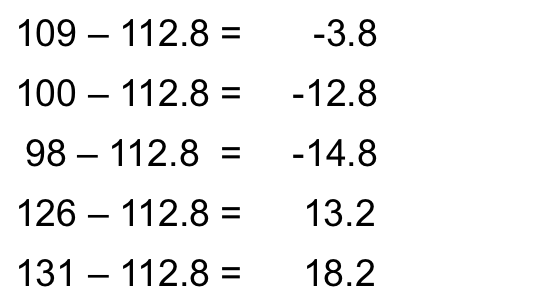
standard deviation example

a note on n-1
Sometimes you will see the formula for standard deviation with only n in the denominator, but technically, this is used for populations.
We use n-1 in samples to note that we are missing information in our sample.
What happens when you increase the number in the denominator of a fraction? Decrease it?
12/4 = 3 or 12/3 = 4
n – 1 makes the denominator smaller and helps us estimate error more accurately (cautiously)
Feeling thermometer example
thinking graphically

dispersion: variance
Variance is very similar to standard deviation but, rather than being the average distance from the average, variance measure the overall distance of the observations from the mean
It is not interpreted in terms of each or any observations, but ALL observations.
In some ways, less informative than standard deviation
No absolute value to look for: larger numbers mean more overall variance in the data, smaller numbers mean less variance
formula for variance

- How is this different than the formula for standard deviation?
- The process for finding the variance is the same as the process for finding the standard deviation except for the last step
- Sometimes the variance is called the “squared standard deviation” hence the notation
variance example
50, 25, 25, 75, 65, 100, 0, 45, 35, 90
choosing the appropriate measure
why stata?
- It is more powerful than other programs, such as SPSS
-
It is less programming oriented than other programs like R
-
Will take a few seminars, but is actually quite straightforward
-
Make use of Acock! And the help menus!