RaiSim Manual
(OUTDATED. Please check our new documentation )
(v.0.6.0)
by Jemin Hwangbo
last updated: 10/29/2019
created: 2/21/2019
Contents
Click the chapters
Intro
Intro: what is RaiSim
RaiSim is a physics engine developed by the researchers at Robotic Systems Lab, ETH Zurich. It was designed to provide both the accuracy and speed for simulating robotic systems. However, it is a generic rigid-body simulator and can simulate any rigid body efficiently.
Intro: why RaiSim?
- The accuracy of RaiSim has been demonstrated through a number of papers ([1], [2])
- The speed is benchmarked against other popular physics engine. (see )
- Easiest C++ simulation library to learn/use
(see ) - A minimum number of dependencies
(only on STL, png, Eigen)
References:
Software Overview
overview
- RaiSim is compiled with gcc-8 and g++-8.
- Dependencies: libpng, libeigen3
- For the latest install instructions, check our github readme
- Currently supported for Ubuntu 16.04 and 18.04
- RaiSim library is without any visualization. For simple rendering, we recommend our opensource package
(https://github.com/leggedrobotics/raisimOgre) - The only header file that you need to include is "raisim/World.hpp"
Software Overview
- Everything in RaiSim is managed by a class called raisim::World. You should not create any other class manually. (except a few math classes, e.g., matrices and vectors)
- RaiSim uses a custom math library for speed. It is rather difficult to use. However, it can be easily converted to its Eigen counterpart (example on the next page)
- Everything is under the namesapce raisim.
- RaiSim has its own version of Open Dynamics Engine (ODE) for collision detection. It is modified in a few different ways.
- Many methods are implemented in the header files so that you can understand exactly what is going on.
Software Overview
Math
- RaiSim offers many Eigen-type front-end methods. However, the backend uses its own math types. The available types are:
Conversion between Eigen and RaiSim types is trivial.
Eigen::VectorXd vectorEigen;
VecDyn vectorRaiSim;

// ... after some algebraic manipulation

// raisim type to eigen type
// (deosn't matter if it is dynamic or static type)
vectorEigen = vectorRaiSim.e();

// eigen type to raisim type
vectorRaiSim = vectorEigen;
raisim::Vec; raisim::VecDyn; raisim::Mat; raisim::MatDyn;
raisim::SparseJacobian; raisim::SparseJacobian1D;Software Overview
Messages
- Raisim has its own logging mechanism. Its design was inspired by glog from Google. It has three different severity levels: INFO, WARN, FATAL. Their corresponding macros are defined as
Prefix "D" can be added. It stands for "Debug" and the log is ignored for release build. For this, add this to your cmake
The purpose of this debug prefix is to prevent unnecessary checks in release mode. You can also add suffix "_IF" if you make it conditional. E.g.,
if (CMAKE_BUILD_TYPE STREQUAL "Debug")
    add_definitions(-DRSDEBUG)
else ()
    remove_definitions(-DRSDEBUG)
endif ()
RSINFO(""), RSWARN(""), RSFATAL("")RSWARN_IF(val<0, "the value is negative")continued on the next page
Software Overview
Messages
The fatal behavior is "exit(1)" by default. You can customize the behavior as
raisim::RaiSimMsg::setFatalCallback([](){throw;});Convention
- Unless otherwise stated explicitly, every quantities in RaiSim is expressed in the world frame and relative to the world frame.
- The world frame has zero acceleration and zero velocity and thus it is an inertial frame
- A quaternion is defined as \( \mathbf{q} = [w, x, y, z]^T\) .
Object: object type
- There are two types of objects: raisim::SingleBodyObject (SB) and raisim::ArticulatedSystem (AS).
- SB is governed by the Newton-Euler equation
-
AS is composed of multiple bodies connected through joints. Each joint defines a constraint. AS is governed by the dynamics equation of a multi-body system
$$\mathbf{M}(\phi)\dot{\mathbf{u}}=\mathbf{\tau}-\mathbf{h}(\mathbf{\phi},\mathbf{u})+\mathbf{J}^T(\mathbf{\phi})\mathbf{f}$$The equation is explained - All objects have a unique world index. The world indices change if an object is removed from the world.
- An object is composed of links. For SB, there is only one link. For AS, there are multiple (>1) links. Each link has a unique index called local index. For SB, local index is always 0.
Object: SingleBodyObject
- Single body objects are created using methods in raisim::World. e.g.,
auto ball = world.addSphere(1, 1); // radius and massObject: Articulated System
- A description of the articulated system should be provided as an urdf file.
- The ROS urdf protocol can be found
- RaiSim urdf protocol differs from the original protocol in four ways
- You can define a capsule as a collision/visual geometry.
- You can define a spherical joint.
- You can define collision material of a collision body. check
chapter for details - Fixed-based systems should have a world link and their first joint is connected to the world link using a fixed joint.
(check the next two pages for details)
- Supported joint types: fixed, revolute, spherical, prismatic
Object: Articulated System
definitions
1. Degrees of freedom: dimension of the minimum representation of the velocity state of a system. Henceforth denoted as \(n\)
2. Generalized velocity: a minimum parameterization of a velocity state of the system (\(\in\mathbb{R}^n\))
3. Generalized coordinate: a parameterization of a configuration of the system (\(\in\mathbb{R}^m\))
4. Generalized state: a generalized velocity and coordinate
(\(\in\mathbb{R}^{n+m}\))
5. Generalized force: external dynamical influences expressed in the generalized velocity space (\(\in\mathbb{R}^{n}\))
Object: Articulated System
Many systems like a robot arm and a cart pole have a fixed-base. A fixed-base should be connected to the link "World" with a fixed joint. For example,
Fixed-base systems
<robot name="2DrobotArm">
    <link name="world"/>

    <link name="link1"/>

    <joint name="worldTolink1" type="fixed">
        <parent link="world"/>
        <child link="link1"/>
        <origin xyz="0 0 0"/>
    </joint>

    <link name="link2">
        <inertial>
            <origin rpy="0 0 0" xyz="0.0 0.0 0.2"/>
            <mass value="1"/>
            <inertia ixx="0.001" ixy="0" ixz="0" iyy="0.001" iyz="0" izz="0.001"/>
        </inertial>
    </link>

    <joint name="link1Tolink2" type="revolute">
        <parent link="link1"/>
        <child link="link2"/>
        <origin xyz="0 0 0.3"/>
        <axis xyz="1 0 0"/>
        <limit effort="80" lower="-1" upper="1" velocity="15"/>
    </joint>
</robot>
Object: Articulated System
For a cart pole, there are four links in the URDF. 1. World 2. the Fixed-base (rail) 3. the cart and 4. the pole. You might be thinking that defining a rail might not be necessary. But such a convention makes the methods in AS consistent for both floating- and fixed- base systems.
Fixed-base systems URDF
Object: Articulated System
generalized coordinate, generalized velocity
- A configuration of the AS can be fully described by a generalized coordinate (GC) \(\mathbf{\phi}\). The minimum parameterization of the velocity state of the AS is called a generalized velocity (GV) \(\mathbf{u}\). The dimension of \(\mathbf{u}\) is called the degrees of freedom (DOF). \(\mathbf{\phi}\) and \(\mathbf{u}\) are a stack of vectors of joint states. In other words, for a robot with \(n\) joints,
***Where \(\phi_i\) and \(u_i\) are GC and GV of each joint. Note that \(\dot{\phi}\) might not be equal to \(\mathbf{u}\)!
Each joint state can also be a vector (for spherical joints)
\(\mathbf{\phi}_i\), \(\mathbf{u}_i\) of different joints. All quantities are expressed in and with respect to the parent frame. For the floating base, the parent is the world frame.
Floating base:
Revolute and prismatic joints:
Spherical joints:
Object: Articulated System
generalized coordinate, generalized velocity
\(\mathbf{\phi}_i\), \(\mathbf{u}_i\) of different joints. All quantities are expressed in and with respect to the parent frame. For the floating base, the parent is the world frame.
Floating base:
Revolute and prismatic joints:
Spherical joints:
Quaternion
Position
Linear velocity
Angular velocity
Quaternion
Angular velocity
Joint position
Joint velocity
Object: Articulated System
generalized coordinate, generalized velocity
Example: pogo stick
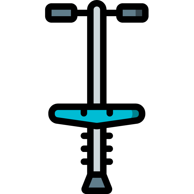
Pogo stick has one prismatic joint and thus two bodies (a floating base and a foot).
Floating base:
prismatic joints:
Object: Articulated System
generalized coordinate, generalized velocity
- The dynamics of AS can be described by the following equation$$\mathbf{M}(\phi)\dot{\mathbf{u}}=\mathbf{\tau}-\mathbf{h}(\mathbf{\phi},\mathbf{u})+\mathbf{J}^T(\mathbf{\phi})\mathbf{f},$$ where \(\mathbf{M}(\phi)\) is the mass matrix, \(\mathbf{\tau}\), is the actuation force/torque, \(\mathbf{h}(\mathbf{\phi},\mathbf{u})\) is a nonlinear term (gravity, coriolis, centrifugal), \(\mathbf{f}\) is the contact forces and \(\mathbf{J}^T(\mathbf{\phi})\) is a stack of their corresponding Jacobians.
- After calling raisim::World::integrate1(), all necessary dynamical quantities for simulation are computed. If you need them for your controller, you can access them as
Eigen::MatrixXd M(robot->getDOF(),robot->getDOF());
Eigen::VectorXd h(robot->getDOF());
M = robot->getMassMatrix();
h = robot->getNonlinearites();
Object: Articulated System
Dynamics quantities
- RaiSim collapses all fixed joints and add their bodies' inertial properties to the parent body. All dynamic properties of a link is defined at the joint connecting the link and its parent.
- RaiSim assigns a local reference frame to every joint. If you want to use a custom frame, define a joint and access the frame as
auto imuFrame = robot->getFrameIdxByName("imu_joint");
raisim::Vec<3> position;
raisim::Mat<3,3> orientation;
robot->getFramePosition(imuFrame, position);
robot->getFrameOrientation(imuFrame, orientation);
Object: Articulated System
Bodies and joints
- RaiSim computes sparse Jacobians of a frame attached to a link. The positional and orientational Jacobians of a point i satisfy the following relationship. $$\mathbf{v}_i=\mathbf{J}^p_i\mathbf{u},$$ $$\mathbf{\omega}_i=\mathbf{J}^o_i\mathbf{u}.$$
- Sparse jacobians are more efficient but more difficult to use. You can use sparse Jacobians directly or just get dense Eigen-type Jacobians instead. Velocity of an arbitrary point can be computed by one of the following ways.
raisim::SparseJacobians jaco;
raisim::VecDyn gv(robot->getDOF());
robot->getSparseJacobian(n, {1,1,1}, jaco);
robot->getGeneralizedVelocity(gv);
raisim::Vec<3> vel;
raisim::matmul(jaco, gv, vel);
Object: Articulated System
(sparse) Jacobians
Eigen::MatrixXd jaco(3, robot->getDOF());
Eigen::VectorXd gv(robot->getDOF());
robot->getDenseJacobian(n, {1,1,1}, jaco);
gv = robot->getGeneralizedVelocity();
Eigen::Vector<3> vel;
vel = jaco * gv;
Sparse (RaiSim) way
Dense (Eigen) way
- RaiSim uses (modified) ODE for collision detection
- Each collision bodies have a name "{link_name}+{/}+{order}"
- Access each collision object as
- For a more efficient access, you can store the iterator as,
robot->getCollisionBodies().get("left_foot/0")->material = "rubber";Object: Articulated System
Collision object
auto colIterator = robot->getCollisionBodies().get("left_foot/0");
colIterator->material = "rubber";
- There are two types of visual objects: real visual objects and collision visual object.
- The best way to understand how to visualize the objects is by reading our Ogre3D-based visualizer code
Object: Articulated System
Visual object
- Raisim provides a stable PD controller (using a custom version of implicit integration). Instead of the explicit version, it computes the average position/velocity error (e.g., $$e=(e_t+e_{t+1})/2$$). It is much more stable than implementing a PD controller yourself.
- The stable PD controller makes a assumption that your PD controller is running at high frequency. If your controller is in fact running at low frequency, this stable PD controller does not reflect the reality very well.
This method uses variables computed for simulation so it minimizes unnecessary computation. - Note that P gain has the dimension equal to the DOF. It produces generalized force which lives in the same space as the generalized velocity.
Object: Articulated System
PD control
- You can also define the rotor inertia in RaiSim. This inertia term is a n-dimensional vector (n is the degrees of freedom). It is directly added to the diagonal of the mass matrix. It also results in more stable simulation. The method to set the rotor inertia is ArticulatedSystem::SetRotorInertia() (currently you cannot set it in URDF)
Object: Articulated System
Rotor inertia
- Since v0.6, you can access Link and Joint using a dedicated API as following
Object: Articulated System
Joint/Link API
raisim::World world;
auto anymal = world->addArticulatedSystem("PATH_TO_URDF");
auto hipJoint = anymal->getJoint("LF_HIP");
raisim::Vec<3> pos;
raisim::Mat<3,3> rot;
hipJoint->getPosition(pos);
hipJoint->getOrientation(rot);

auto shank = anymal->getLink("LF_SHANK");
shank.setComPositionInParentFrame({0., 1.0, 0.0}); // change dynamic properties online

world->integrate();
1. Detailed example can be found in "creatingRobotUsingCPP" example in raisimOgre
2. raisim::World class has addAritculatedSystem(const Child &, ...) method. raisim::Child is a class that defines a kinematic tree. It contains a body, a joint and Children (a group of Child). Children are either child or fixedBodies. child can move with respect to the parent, fixedBodies cannot (and therefore contains a fixed joint).
A body can have multiple CollisionBody's and VisObject. All bodies and joints must have a unique name
Object: Articulated System
Programmatically create an articulated system
Object: body type
- There are three different body types: Dynamic, Kinematic, Static. A static object (e.g., ground) has an infinite mass and cannot move. A kinematic object (e.g., conveyor belt) has an infinite mass but still can move kinematically (with a specified velocity). A dynamic object (e.g., a ball) has a finite mass and can move.
- Two non-dynamic (static or kinematic) objects cannot collide each other.
- All objects have a default body type. For a SingleBodyObject, you can override it manually as following:
sphere->setBodyType(raisim::BodyType::STATIC);Constraints
- Currently supports only Stiff Wire. Compliant Wire will be added soon. Stiff Wire is a unilateral constraint in the velocity space. It can bend if compressed but it cannot stretch (but numerical error can occur). Check out "raisimOgre/examples/src/primitives/newtonsCradle.cpp" for details.
Material system
- All material properties are defined over a pair. So if you defined 4 different materials, there are total of 10 (=4+3+2+1) materials property sets.
- If you don't define material pair properties, the default parameter is $$\mu=0.8, \epsilon=0, \widehat{\epsilon}=0,$$ where \( \mu\) is the coefficient of friction, \( \epsilon\) is the coefficient of restitution, and \( \widehat{\epsilon}\) is the threshold of restitution.
- Friction dynamics is explained in [1], the restitution dynamics is defined as the graph on the next page.
- Material properties can be provided by an xml file (e.g.,"examples/rsc/basicMaterials.xml") or in the code (e.g., "examples/src/primitives/newtonsCradle.cpp")
References:
Continued on the next page
Material system
restitution
Bouncing
velocity
Impact
velocity
\( \widehat{\epsilon}\)
\( \epsilon\)
Continued on the next page
How to define material prooperties
Continued on the next page
- Material properties can be provided by an xml file (e.g.,"examples/rsc/basicMaterials.xml") or in the code (e.g., "examples/src/primitives/newtonsCradle.cpp")
- You can also dynamically define material properties
- If you don't want to define material properties for every pairs, you can simply set the default property
raisim::World->setMaterialPairProp("steel","aluminum", 0.8, 0., 0.);raisim::World->setDefaultMaterial(0.8, 0., 0.);How to assign material to an object.
Continued on the next page
- For raisim::AriticulatedSystem, materials are defined in the corresponding urdf file (in link/collision/material/contact). E.g.,
You can also programatically set the material, e.g.,
note that collision bodies have a name "LINK_NAME/X", where X is the number assigned for collision bodies
<link name="base_inertia">
    <collision>
        <origin rpy="1.57079632679 0 0" xyz="0.0 0.07 -0.25"/>
        <geometry>
            <cylinder length="0.08" radius="0.04"/>
        </geometry>
        <material>
            <contact name="steel"/>
        </material>
    </collision>
</link>robot->getCollisionBody("base/0").setMaterial("steel");How to assign material to an object.
Continued on the next page
2. For raisim::SingleBodyObject, material properties are defined at instantiation. E.g.,
If not material is assigned, gets default material "" (empty) and it will have the default material property
world.addSphere(1., 1., "steel");Contact
1. RaiSim uses a standard way to filter out unwanted collision, using collision groups and collision masks. Each object belongs to one or multiple collision groups and contains a collision mask. Both collision groups and masks are unsigned long int and can be interpreted as 32-long bit field.
The collision logic is as follows:
Collision group and collision mask
if( (ObjectA->collisionGroup & ObjectB->collisionMask) ||
    (ObjectB->collisionGroup & ObjectA->collisionMask) )
  collide();
Contact
1. Information on contacts on an object can be obtained using Object::getContact(). If this method is called before raisim::World::integrate1(), the contacts are for the last time steps. If it is called after the raisim::World::integrate1(), the contacts are for the current time step
2. When two objects collide, one of them is called "objectA" and the other is called "objectB". The contact impulse is defined in the contact frame of "objectA" and its z-axis is into "objectA". It is also called a contact normal (perpendicular to the surface). The choice of the X-axis and the Y-axis of a contact frame is arbitrary.
Contact
1. RaiSim has an algorithm to remove object inter-penetrations which can arise due to numerical errors. It adds a spring and a damping term. The spring stiffness is determined such that the contact point has a separating velocity of erp1 times the depth of the penetration. The damping coefficient is exactly equivalent to the restitution coefficient and the effective restitution coefficient is erp2 + the original restitution coefficient of the material pair. The erp1 and erp2 are global and specified in the world.
Error reduction
World system
raisim::World class manages all resources. Currently, you can only dynamically generate the world. We are working on a method of generating a world from a script.
World system
Users can dynamically add or remove objects in RaiSim. However, add or remove object methods should not be called between integrate1() and integrate2() calls.
Dynamic world editing
Visualizer
Raisim is a physics engine and does not contain any visualizer. However, we provide an open-source visualizer based on Ogre3d, which can be found at
RaiSim for Reinforcement Learning
We provide an open-source example of RL using raisim at
Python binding
A python wrapper developed by Brian Delhaisse is available here:
Examples
#include “raisim/World.hpp”

int main() {
    raisim::World world;
    auto anymal = world.addArticulatedSystem(“pathToURDF”);
    auto ball = world.addSphere(1, 1); // radius and mass
    auto ground = world.addGround();

    world.setTimeStep(0.002);
    world.integrate();
}
The following code simulates a robot and a sphere on a flat ground for one time step