Hopping through parameter space with XSEC

Jeriek Van den Abeele

Monash University

Based on arXiv:2006.16273

@JeriekVda

Outline

Global fits and the need for speed
Gaussian Processes 101
Beyond basics: scaling up
Validation results
Getting started with XSEC

1. Global fits and the need for speed

Many experiments

Many theories

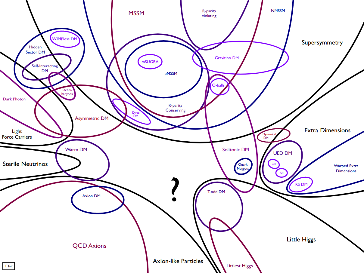
Many experiments

Many theories

Many observables

measurements

predictions

Global fits address the need for a consistent comparison of theories to all available experimental data

Challenge:

Scanning increasingly high-dimensional parameter spaces with varying phenomenology

$\mathcal{L} = \mathcal{L}_\mathsf{collider} \times \mathcal{L}_\mathsf{Higgs} \times \mathcal{L}_\mathsf{DM} \times \mathcal{L}_\mathsf{EWPO} \times \mathcal{L}_\mathsf{flavour} \times \ldots$

Global fits need quick, but sufficiently accurate theory predictions

BSM scans today already require $\sim 10^7$ samples

Calculating higher-order BSM production cross-sections and theoretical uncertainties makes a difference ... but it takes too long!

Prospino/MadGraph: ~ minutes/hours
N(N)LL-fast: only degenerate squarks

[GAMBIT, 1705.07919]

CMSSM

[hep-ph/9610490]

$$ pp\to\tilde g \tilde g,\ \tilde g \tilde q_i,\ \tilde q_i \tilde q_j, $$

$$\tilde q_i \tilde q_j^{*},\ \tilde b_i \tilde b_i^{*},\ \tilde t_i \tilde t_i^{*}$$

at NLO, at $\mathsf{\sqrt{s}=13} $ TeV

with PDF, $\alpha_s$ and scale uncertainty

xsec 1.0 performs smart regression for

QCD ... still going strong

2. Gaussian Processes 101

$$$

CPU time is money ...

Interpolation ...

Interpolation ... doesn't give prediction uncertainty!

Correlation length-scale

Estimate from data!

Correlation length-scale

Estimate from data!

Correlation length-scale

Gaussian process prediction with uncertainty

Estimate from data!

prior distribution over all functions

with the estimated smoothness

f(\vec x) \sim \mathcal{GP}\left[m(\vec x), k(\vec x, \vec x')\right]

\mathrm{E}\left[f(\vec x)\right] = m(\vec x)

\mathrm{Cov}\left[f(\vec x), f(\vec x')\right] = k(\vec x, \vec x')

The Bayesian Way: quantify your beliefs about the target function with probabilities

k(\vec x, \vec x') = \sigma_f^2 \exp\left(-\frac{|\vec x-\vec x'|^2}{2 l^2}\right)

prior distribution over all functions

with the estimated smoothness

f(\vec x) \sim \mathcal{GP}\left[m(\vec x), k(\vec x, \vec x')\right]

\mathrm{E}\left[f(\vec x)\right] = m(\vec x)

\mathrm{Cov}\left[f(\vec x), f(\vec x')\right] = k(\vec x, \vec x')

The Bayesian Way: quantify your beliefs about the target function with probabilities

k(\vec x, \vec x') = \sigma_f^2 \exp\left(-\frac{|\vec x-\vec x'|^2}{2 l^2}\right)

posterior distribution over functions

with updated $m(\vec x)$

data

Let's make some draws from this prior distribution

At each input point, we obtain a distribution of possible function values (prior to looking at data)

A Gaussian process sets up an infinite number of correlated Gaussians, one at each parameter point

We obtain a posterior by conditioning on known data

target function

We obtain a posterior by conditioning on known data

target function

We obtain a posterior by conditioning on known data

Make posterior predictions at new points by computing correlations to known points

Posterior predictive distributions are Gaussian too

Squared Exponential kernel

Matérn-3/2 kernel

Different kernels lead to different function spaces to marginalise over

My kingdom for a good kernel ...

GPs allow us to use probabilistic inference to learn a function from data, in an interpretable, analytical, yet non-parametric Bayesian framework.

A GP model is fully specified once the mean function, the kernel and its hyperparameters are chosen.

The probabilistic interpretation only holds under the assumption that the chosen kernel accurately describes the true correlation structure.

The choice of kernel allows for great flexibility. But once chosen, it fixes the type of functions likely under the GP prior and determines the kind of structure captured by the model, e.g., periodicity and differentiability.

[D. Duvenaud, PhD thesis]

My kingdom for a good kernel ...

[D. Duvenaud, PhD thesis]

My kingdom for a good kernel ...

[D. Duvenaud, PhD thesis]

My kingdom for a good kernel ...

For our multi-dimensional case of cross-section regression, we get good results by multiplying Matérn ($\nu = 3/2$) kernels over the different mass dimensions:

\displaystyle k_s(\vec x, \vec x') = \prod_{d=1}^D \sigma_{f_d}^2 \left( 1 + \sqrt{3} \frac{|x'_d - x_d|}{l_d} \right) \exp\left(-\sqrt{3}\frac{|x'_d - x_d|}{l_d}\right)

The different lengthscale parameters $l_d$ lead to automatic relevance determination for each feature: short-range correlations for important features over which the target function varies strongly.

This is an anisotropic, stationary kernel. It allows for functions that are less smooth than with the standard squared-exponential kernel.

[Deisenroth+, Distill.pub]

My kingdom for a good kernel ...

... with good hyperparameters

Short lengthscale, small noise

Long lengthscale, large noise

Underfitting, almost linear

Overfitting of fluctuations,

[Deisenroth+, Distill.pub]

can lead to large uncertainties!

Typically, kernel hyperparameters are estimated by maximising the (log) marginal likelihood $p( \vec y\ |\ \vec X, \vec \theta) $, aka the empirical Bayes method.

Alternative: MCMC integration over a range of $\vec \theta$.

Gradient-based optimisation can get stuck in local optima and plateaus. Multiple initialisations can help, or global optimisation methods like differential evolution.

Global optimum: somewhere in between

[Deisenroth+, unpublished]

... with good hyperparameters

Typically, kernel hyperparameters are estimated by maximising the (log) marginal likelihood $p( \vec y\ |\ \vec X, \vec \theta) $, aka the empirical Bayes method.

Alternative: MCMC integration over a range of $\vec \theta$.

Gradient-based optimisation can get stuck in local optima and plateaus. Multiple initialisations can help, or global optimisation methods like differential evolution.

The standard approach systematically underestimates prediction errors.

After accounting for the additional uncertainty from learning the hyper-parameters, the prediction error increases when far from training points.

[Wågberg+, 1606.03865]

... with good hyperparameters

Other tricks to improve the numerical stability of training:

Normalising features and target values
Factoring out known behaviour from the target values
Training on log-transformed targets, for extreme values and/or a large range, or to ensure positive predictions

... with good hyperparameters

Workflow

Generating data

Random sampling

SUSY spectrum

Cross sections

Optimise kernel hyperparameters

Training GPs

GP predictions

Input parameters

Linear algebra

Cross-section

estimates

Compute covariances

Workflow

Generating data

Random sampling

SUSY spectrum

Cross sections

Optimise kernel hyperparameters

Training GPs

GP predictions

Input parameters

Linear algebra

Cross-section

estimates

Compute covariances

XSEC

3. Beyond basics: scaling up

Training scales as $\mathcal{O}(n^3)$, prediction as $\mathcal{O}(n^2)$

A balancing act

Mix of random samples with different priors in mass space

Evaluation speed

Sample coverage

Need to cover a large parameter space

Distributed Gaussian processes

[Liu+, 1806.00720]

Generalized Robust Bayesian Committee Machines

Aggregation model for dealing with large datasets

Split the data into 1 global communication set $\mathcal D_c$ and any number of local expert sets $\mathcal D_i$
Train a separate GP on each data set
Augment $\mathcal D_i$ with $\mathcal D_c$ , without re-training
Combine predictions from the separate GPs, giving larger weight to experts with small uncertainty

Sometimes, a curious problem arises: negative predictive variances!

It is due to numerical errors when computing the inverse of the covariance matrix $K$. When $K$ contains many training points, there is a good chance that some of them are similar:

\vec x_1 \sim \vec x_2 \quad \implies \quad k(\vec x_1, \vec X) \simeq k(\vec x_2, \vec X)

GP regularisation

Nearly equal columns make $K$ ill-conditioned. One or more eigenvalues $\lambda_i$ are close to zero and $K$ can no longer be inverted reliably. The number of significant digits lost is roughly the $\log_{10}$ of the condition number

\kappa = \frac{\lambda_\mathsf{max}}{\lambda_\mathsf{min}}

This becomes problematic when $\kappa \gtrsim 10^8 $. In the worst-case scenario,

\kappa = N \left(\frac{\sigma_f}{\sigma_n}\right)^2 + 1

signal-to-noise ratio

number of points

[Deisenroth+, Distill.pub]

GP regularisation

Add a white-noise component to the kernel
- Can compute minimal value that reduces $\kappa$ sufficiently
- Can model discrepancy between GP model and latent function, e.g., regarding assumptions of stationarity and differentiability

[Deisenroth+, Distill.pub]

[Mohammadi+, 1602.00853]

Avoid a large S/N ratio by adding a likelihood penalty term guiding the hyperparameter optimisation
- Nearly noiseless data is problematic ... Artificially increasing the noise level may be necessary, degrading the model a bit

4. Validation results

Gluino-gluino

Gluino-squark

Squark-squark

Squark-antisquark

5. Getting started with XSEC

github.com/jeriek/xsec

pip install xsec
xsec-download-gprocs --process_type gg

# Set directory and cache choices
xsec.init(data_dir="gprocs")

# Set center-of-mass energy (in GeV)
xsec.set_energy(13000)

# Load GP models for the specified process(es)
processes = [(1000021, 1000021)]
xsec.load_processes(processes)

# Enter dictionary with parameter values
xsec.set_parameters(
    {
        "m1000021": 1000,
        "m1000001": 500,
        "m1000002": 500,
        "m1000003": 500,
        "m1000004": 500,
        "m1000005": 500,
        "m1000006": 500,
        "m2000001": 500,
        "m2000002": 500,
        "m2000003": 500,
        "m2000004": 500,
        "m2000005": 500,
        "m2000006": 500,
        "sbotmix11": 0,
        "stopmix11": 0,
        "mean": 500,
    }
)

# Evaluate the cross-section with the given input parameters
xsec.eval_xsection()

# Finalise the evaluation procedure
xsec.finalise()

More at the TOOLS workshop next week!

Fast estimate of SUSY (strong) production cross- sections at NLO, and uncertainties from

regression itself
renormalisation scale
PDF variation
$\alpha_s$ variation

Goal

$$ pp\to\tilde g \tilde g,\ \tilde g \tilde q_i,\ \tilde q_i \tilde q_j, $$

$$\tilde q_i \tilde q_j^{*},\ \tilde b_i \tilde b_i^{*},\ \tilde t_i \tilde t_i^{*}$$

Interface

Method

Pre-trained, distributed Gaussian processes

Stand-alone Python tool

Processes

at $\mathsf{\sqrt{s}=13}$ TeV

Available at github.com/jeriek/xsec

arXiv:2006.16273

Thank you!

Backup slides

All the scary math

Regression problem, with 'measurement' noise:

$y=f(\vec x) + \varepsilon, \ \varepsilon\sim \mathcal{N}(0,\sigma_n^2) \quad \rightarrow \quad $ infer $f$, given data $\mathcal{D} = \{\vec X, \vec y\}$

Assume covariance structure expressed by a kernel function, like

k(\vec x_i, \vec x_j) = \sigma_f^2\, \exp\!\left(-\frac{|\vec x_i - \vec x_j|^2}{2\mathcal{l}^2}\right) + \sigma_n^2\, \delta_{ij}

Consider the data as a sample from a multivariate Gaussian distribution

$[\vec x_1, \vec x_2, \ldots]$

$[y_1, y_2, \ldots]$

signal kernel

white-noise kernel

All the scary math

Regression problem, with 'measurement' noise:

$y=f(\vec x) + \varepsilon, \ \varepsilon\sim \mathcal{N}(0,\sigma_n^2) \quad \rightarrow \quad $ infer $f$, given data $\mathcal{D} = \{\vec X, \vec y\}$

Training: optimise kernel hyperparameters by maximising the marginal likelihood

p\left( \vec y\ |\ \vec X, \vec \theta \right) = \mathcal{N} \left( \vec y \ |\ m(\vec X), K_{\vec\theta} \right)

y_*\, |\, \mathcal D, \vec x_* \sim \mathcal{N}\left(\mu_*, \sigma_*^2\right)

\propto |K_{\vec\theta}|^{-\frac{1}{2}} \times \exp \left\{ -\frac{1}{2} \left( \vec y - m(\vec X) \right)^T K_{\vec\theta}^{-1} \left(\vec y - m(\vec X) \right) \right\} % %%k(\vec X, \vec X)^{-1} \left( \vec y - \mu(\vec X) \right), % k(\vec x_*, \vec x_*) - k(\vec x_*, \vec X) k(\vec X, \vec X)^{-1} k(\vec X, \vec x_*)

Posterior predictive distribution at a new point $\vec x_*$ :

with

\mu_* = m(\vec x_*) + K_* K^{-1}(\vec{y}-m(\vec X)) %%\tilde\mu(\vec x_*) = \mu(\vec x_*) + k(\vec x_*, \vec X) k(\vec X, \vec X)^{-1}\vec{y}\\ %\tilde\sigma^2(\vec x_*) = k(\vec x_*, \vec x_*) - k(\vec x_*, \vec X) k(\vec X, \vec X)^{-1} k(\vec X, \vec x_*)

Implicit integration over points not in $\vec X$

\sigma_*^2 = K_{**}-K_*K^{-1}K_*^T %%\tilde\mu(\vec x_*) = \mu(\vec x_*) + k(\vec x_*, \vec X) k(\vec X, \vec X)^{-1}\vec{y}\\ %\tilde\sigma^2(\vec x_*) = k(\vec x_*, \vec x_*) - k(\vec x_*, \vec X) k(\vec X, \vec X)^{-1} k(\vec X, \vec x_*)

[

K = k(\vec X, \vec X) \\ K_* = k(x_*, \vec X) \\ K_{**} = k(\vec x_*, \vec x_*)

Gaussian Processes 101 (non-parametric regression)

prior over functions

The covariance matrix controls smoothness.

Assume it is given by a kernel function, like

k(x_1, x_2) = \exp\!\left(-\frac{|x_2-x_1|^2}{2\mathcal{l}^2}\right).

posterior over functions

Bayesian approach to estimate $ y_* = f(x_*) $ :

y_* | \mathbf{y} \sim \mathcal{N}(K_* K^{-1}\mathbf{y},\ K_{**}-K_*K^{-1}K_*^T)

Consider the data as a sample from a multivariate Gaussian distribution.

\begin{pmatrix} \mathbf{y} \\ y_{*} \end{pmatrix} \sim \mathcal{N}{\left( \begin{pmatrix} \mathbf{0} \\ 0 \end{pmatrix} , \begin{bmatrix} K & K_{*}\\ K_{*}^T & K_{**}\\ \end{bmatrix} \right)}

K_{ij} = k(x_i, x_j) \\ K_{*i}= k(x_*,x_i) \\ K_{**} = k(x_*,x_*)

data

mean

covariance

Gaussian Processes 101 (non-parametric regression)

prior over functions

The covariance matrix controls smoothness.

Assume it is given by a kernel function, like

k(x_1, x_2) = \exp\!\left(-\frac{|x_2-x_1|^2}{2\mathcal{l}^2}\right).

posterior over functions

Bayesian approach to estimate $ y_* = f(x_*) $ :

y_* | \mathbf{y} \sim \mathcal{N}(K_* K^{-1}\mathbf{y},\ K_{**}-K_*K^{-1}K_*^T)

Consider the data as a sample from a multivariate Gaussian distribution.

\begin{pmatrix} \mathbf{y} \\ y_{*} \end{pmatrix} \sim \mathcal{N}{\left( \begin{pmatrix} \mathbf{0} \\ 0 \end{pmatrix} , \begin{bmatrix} K & K_{*}\\ K_{*}^T & K_{**}\\ \end{bmatrix} \right)}

K_{ij} = k(x_i, x_j) \\ K_{*i}= k(x_*,x_i) \\ K_{**} = k(x_*,x_*)

data

mean

covariance

Radial Basis Function kernel

prior over functions

The covariance matrix controls smoothness.

Assume it is given by a kernel function, like

k(x_1, x_2) = \exp\!\left(-\frac{|x_2-x_1|^2}{2\mathcal{l}^2}\right).

posterior over functions

Bayesian approach to estimate $ y_* = f(x_*) $ :

y_* | \mathbf{y} \sim \mathcal{N}(K_* K^{-1}\mathbf{y},\ K_{**}-K_*K^{-1}K_*^T)

Consider the data as a sample from a multivariate Gaussian distribution.

\begin{pmatrix} \mathbf{y} \\ y_{*} \end{pmatrix} \sim \mathcal{N}{\left( \begin{pmatrix} \mathbf{0} \\ 0 \end{pmatrix} , \begin{bmatrix} K & K_{*}\\ K_{*}^T & K_{**}\\ \end{bmatrix} \right)}

K_{ij} = k(x_i, x_j) \\ K_{*i}= k(x_*,x_i) \\ K_{**} = k(x_*,x_*)

data

mean

covariance

Matérn kernel

Gaussian Processes 101 (non-parametric regression)

Scale-dependence of LO/NLO

[Beenakker+, hep-ph/9610490]