Accelerating new physics searches with XSEC
Jeriek Van den Abeele
Spåtind 2020
Skeikampen – January 6
Based on work with A. Buckley,
I.A.V. Holm, A. Kvellestad,
A. Raklev, P. Scott,
J.V. Sparre


@JeriekVda


$$$
Time is money


Interpolation ...

Interpolation ... doesn't give prediction uncertainty!


Correlation length-scale
Correlation length-scale

Correlation length-scale
Correlation length-scale
Correlation length-scale
Correlation length-scale
Correlation length-scale
Correlation length-scale
Correlation length-scale
Estimate from data! (kernels)

Correlation length-scale
Estimate from data! (kernels)

Correlation length-scale
Gaussian process prediction with uncertainty
Estimate from data! (kernels)
Correlation length-scale
Gaussian process prediction with uncertainty
Estimate from data! (kernels)


Gaussian Processes 101
prior over all functions
with the estimated smoothness
posterior over functions
data
Radial Basis Function kernel

Gaussian Processes 101
prior over all functions
with the estimated smoothness
posterior over functions
data
Matérn kernel
New physics? Yes, please!

Global fits and the need for speed
Idea: consistent comparison of theories to all available data
- High-dimensional parameter space with varying phenomenology (e.g. MSSM-24)
- Quick prediction of next-to-leading order cross sections is crucial!
- Existing tools have drawbacks (Prospino: slow, NLL-fast: limited validity)
\(\mathcal{L} = \mathcal{L}_\mathsf{collider} \times \mathcal{L}_\mathsf{Higgs} \times \mathcal{L}_\mathsf{DM} \times \mathcal{L}_\mathsf{EWPO} \times \mathcal{L}_\mathsf{flavour} \times \ldots\)

[GAMBIT, 1705.07919]
CMSSM


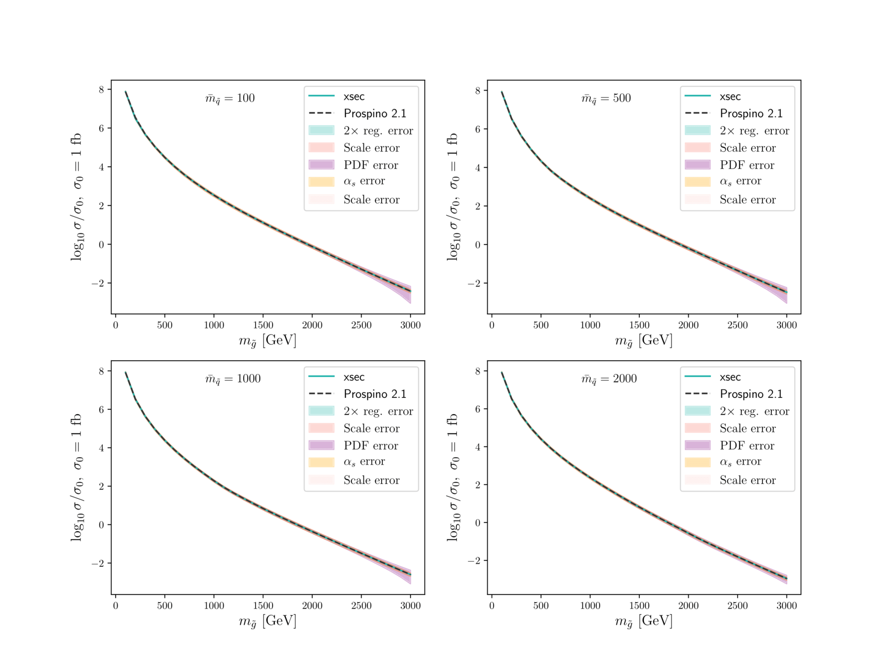
Fast estimate of SUSY (strong) production cross sections at NLO, and uncertainties from
- regression itself
- renormalisation scale
- PDF variation
- \(\alpha_s\) variation
Goal
$$ pp\to\tilde g \tilde g,\ \tilde g \tilde q_i,\ \tilde q_i \tilde q_j, $$
$$\tilde q_i \tilde q_j^{*},\ \tilde b_i \tilde b_i^{*},\ \tilde t_i \tilde t_i^{*}$$
Interface
Method
Pre-trained, distributed Gaussian processes
Stand-alone Python code, also implemented in GAMBIT
Processes

at \(\mathsf{\sqrt{s}=7/8/13/14}\) TeV
Soon public on GitHub!
Workflow
Generating data
Random sampling
SUSY spectrum
Cross sections
Optimise kernel hyperparameters
Training GPs
GP predictions
Input parameters
Linear algebra
Cross section
estimates
Compute covariances
Workflow
Generating data
Random sampling
SUSY spectrum
Cross sections
Optimise kernel hyperparameters
Training GPs
GP predictions
Input parameters
Linear algebra
Cross section
estimates
Compute covariances
XSEC
Training scales as \(\mathcal{O}(n^3)\), prediction as \(\mathcal{O}(n^2)\)

A balancing act
Mix of random samples with different priors in mass space
Evaluation speed
Sample coverage
Need to cover a large parameter space
Distributed Gaussian processes
Training scales as \(\mathcal{O}(n^3)\), prediction as \(\mathcal{O}(n^2)\)
A balancing act
Mix of random samples with different priors in mass space
Evaluation speed
Sample coverage
Need to cover a large parameter space
Distributed Gaussian processes

[Liu+, 1806.00720]
Generalized Robust Bayesian Committee Machine
Plots, plots, plots
XSEC: the cross-section evaluation code

XSEC: the cross-section evaluation code

XSEC: the cross-section evaluation code
XSEC: the cross-section evaluation code

XSEC: the cross-section evaluation code


XSEC: the cross-section evaluation code
Thank you!


Backup slides
Gaussian Processes 101 (non-parametric regression)
prior over functions

The covariance matrix controls smoothness.
Assume it is given by a kernel function, like
posterior over functions
Bayesian approach to estimate \( y_* = f(x_*) \) :
Consider the data as a sample from a multivariate Gaussian distribution.
data
mean
covariance
Gaussian Processes 101 (non-parametric regression)
prior over functions
The covariance matrix controls smoothness.
Assume it is given by a kernel function, like
posterior over functions
Bayesian approach to estimate \( y_* = f(x_*) \) :
Consider the data as a sample from a multivariate Gaussian distribution.
data
mean
covariance
Radial Basis Function kernel
prior over functions
The covariance matrix controls smoothness.
Assume it is given by a kernel function, like
posterior over functions
Bayesian approach to estimate \( y_* = f(x_*) \) :
Consider the data as a sample from a multivariate Gaussian distribution.
data
mean
covariance
Matérn kernel
Gaussian Processes 101 (non-parametric regression)
XSEC: the cross section evaluation code
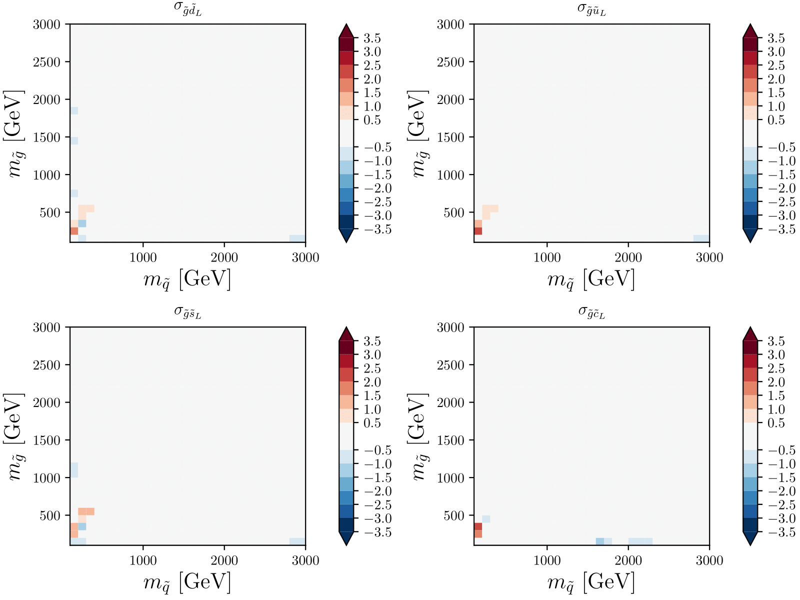
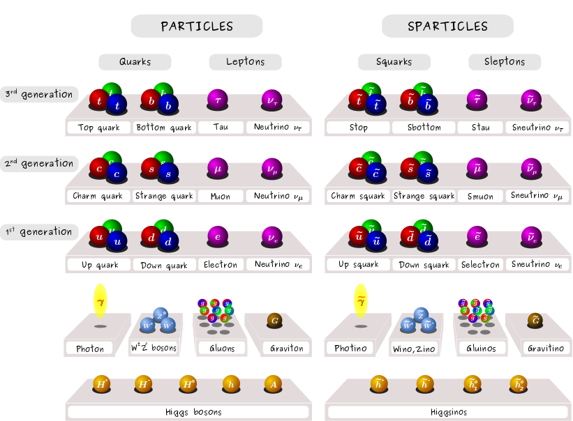
Image: Claire David (CERN)

Scale-dependence of LO/NLO
[Beenakker+, hep-ph/9610490]