

Sponsors
Please join the BTVDataScience Group on Datacamp!

You!!!
Bayesian Inference Made Easy*

*Easier. User caution still advised.
John Stanton-Geddes
18 May 2016
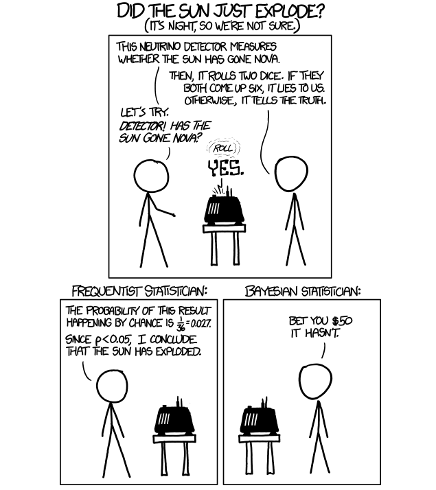
http://xkcd.com/1132/
Frequentist
- probabilities are related to frequency of the observed sample from many repeated samples drawn from same underlying distribution
- parameters have a fixed value
yields
- point estimates
- confidence intervals
Frequentist Confidence Intervals
Interactive Demo by Nick Strayer
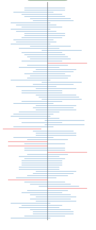
95% of the intervals generated with a sample drawn from the underlying distribution will include the true value of the parameter
Bayesian Inference
- probabilities are related to prior information and updated by available data
- parameter values treated as random, drawn from prior distribution
yields
- posterior intervals
Bayes' Billiards Table

Bayes' Billiards Table
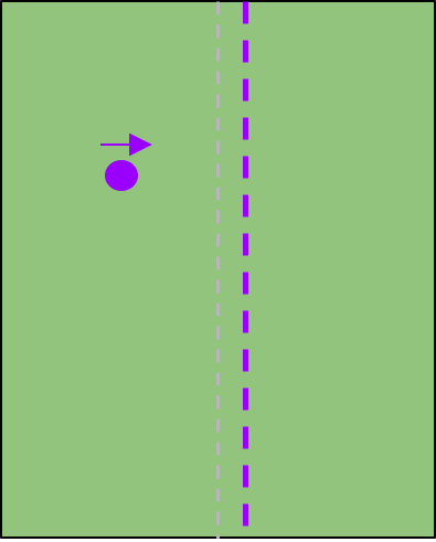
Bayes' Billiards Table
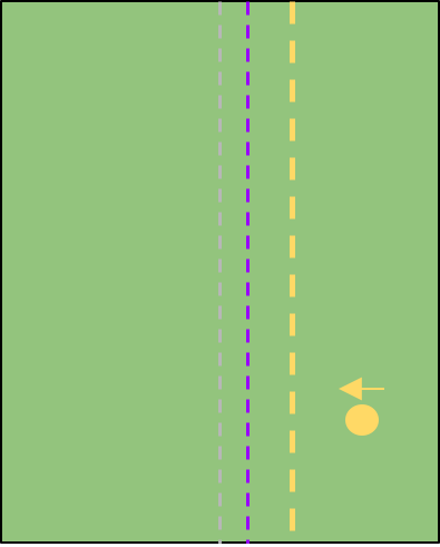
Bayes' Billiards Table
There are several reasons why everyone isn’t using Bayesian methods for regression modeling. One reason is that Bayesian modeling requires more thought: you need pesky things like priors, and you can’t assume that if a procedure runs without throwing an error that the answers are valid.
https://thinkinator.com/2016/01/12/r-users-will-now-inevitably-become-bayesians/
There are several reasons why everyone isn’t using Bayesian methods for regression modeling. One reason is that Bayesian modeling requires more thought: you need pesky things like priors, and you can’t assume that if a procedure runs without throwing an error that the answers are valid. A second reason is that MCMC sampling — the bedrock of practical Bayesian modeling — can be slow compared to closed-form or MLE procedures.
https://thinkinator.com/2016/01/12/r-users-will-now-inevitably-become-bayesians/
There are several reasons why everyone isn’t using Bayesian methods for regression modeling. One reason is that Bayesian modeling requires more thought: you need pesky things like priors, and you can’t assume that if a procedure runs without throwing an error that the answers are valid. A second reason is that MCMC sampling — the bedrock of practical Bayesian modeling — can be slow compared to closed-form or MLE procedures. A third reason is that existing Bayesian solutions have either been highly-specialized (and thus inflexible), or have required knowing how to use a generalized tool like BUGS, JAGS, or Stan. This third reason has recently been shattered in the R world by not one but two packages: brms and rstanarm.
https://thinkinator.com/2016/01/12/r-users-will-now-inevitably-become-bayesians/

http://mc-stan.org/interfaces/rstanarm
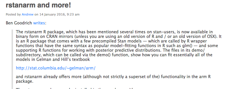
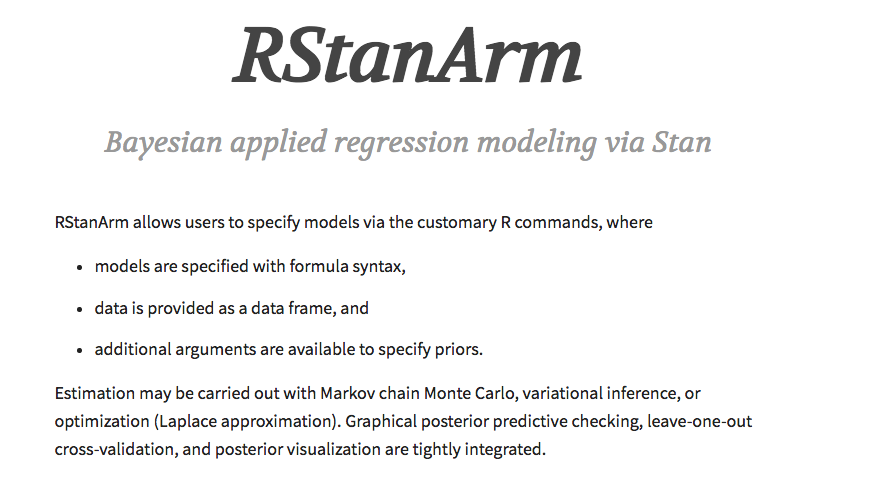
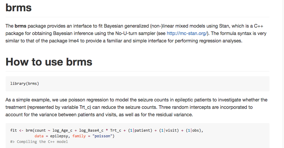
https://github.com/paul-buerkner/brms
Ice Cream Sales
example borrowed from
http://www.magesblog.com/2015/08/visualising-theoretical-distributions.html
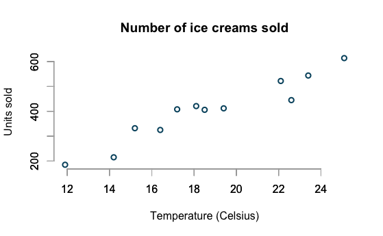
Log-linear model
> log_lin_mod <- glm(log(units) ~ temp, data=icecream,
+ family=gaussian(link="identity"))
> arm::display(log_lin_mod)
glm(formula = log(units) ~ temp, family = gaussian(link = "identity"),
    data = icecream)
            coef.est coef.se
(Intercept) 4.40     0.20
temp        0.08     0.01
---
  n = 12, k = 2
  residual deviance = 0.2, null deviance = 1.4 (difference = 1.2)
  overdispersion parameter = 0.0
  residual sd is sqrt(overdispersion) = 0.14
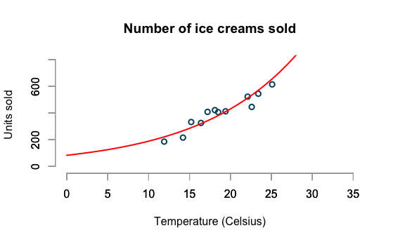
Log-linear model
Stan
stanLogTransformed <-"
data {
  int N;
  vector[N] units;
  vector[N] temp;
}
transformed data {
  vector[N] log_units;
  log_units <- log(units);
}
parameters {
  real alpha;
  real beta;
  real tau;
}
transformed parameters {
  real sigma;
  sigma <- 1.0 / sqrt(tau);
}
model{
  // Model
  log_units ~ normal(alpha + beta * temp, sigma);
  // Priors
  alpha ~ normal(0.0, 1000.0);
  beta ~ normal(0.0, 1000.0);
  tau ~ gamma(0.001, 0.001);
}
generated quantities{
  vector[N] units_pred;
  for(i in 1:N)
    units_pred[i] <- exp(normal_rng(alpha + beta * temp[i], sigma));
}
"
Specify the model in Stan DSL
Stan
temp <- c(11.9,14.2,15.2,16.4,17.2,18.1,18.5,19.4,22.1,22.6,23.4,25.1)
units <- c(185L,215L,332L,325L,408L,421L,406L,412L,522L,445L,544L,614L)
library(rstan)
stanmodel <- stan_model(model_code = stanLogTransformed)
fit <- sampling(stanmodel,
                data = list(N=length(units),
                            units=units,
                            temp=temp),
                iter = 1000, warmup=200)
stanoutput <- extract(fit)

## Extract estimated parameters
(parms <- sapply(stanoutput[c("alpha", "beta", "sigma")], mean))


     alpha       beta      sigma
4.39065304 0.08315599 0.14995194
Run in R
RStanARM
ic4 <- stan_glm(log(units) ~ temp, data = icecream,
    family = gaussian(link = "identity"))

> ic4
stan_glm(formula = log(units) ~ temp,
    family = gaussian(link = "identity"),
    data = icecream)

Estimates:
            Median MAD_SD
(Intercept) 4.4    0.2
temp        0.1    0.0
sigma       0.1    0.0

Sample avg. posterior predictive
distribution of y (X = xbar):
         Median MAD_SD
mean_PPD 5.9    0.1
Fit the same model, using R formula syntax!
Using RStanARM
- Specify a joint distribution for the outcomes and unknowns.
- Draw from the posterior distribution using MCMC
- Evaluate model fit
- Predict using draws from the posterior predictive distribution to visualize impact of predictors
Digital Workflow A/B Testing
Can we use Bayesian inference through RStanARM to test variants of website design while:
- 'peeking' at results
- avoiding inflated false positive rate
- minimizing complexity of code
- facilitating agile analysis
Digital Workflow A/B Testing
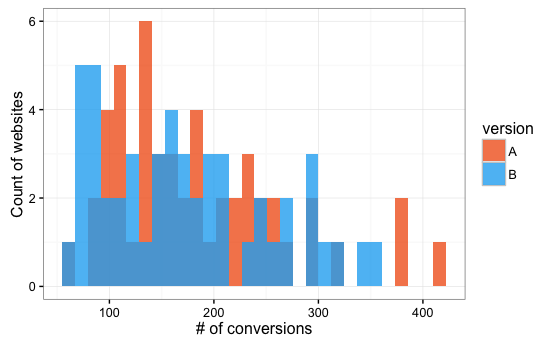
1,000 simulated datasets with both variants drawing from
log-normal distribution
Digital Workflow A/B Testing
Of 1,000 simulated data sets,
51 linear models had P < 0.05 and
28 Bayesian models had 95% credible intervals > 0.
Here Be Dragons
slm1 <- stan_lm(log(conversions) ~ version, data = sim_dat,
                prior = R2(what = "mean", location = 0.1))
slm1

slm1_ci95 <- posterior_interval(slm1, prob = 0.95, pars = "versionB")
round(exp(slm1_ci95), 2)


         2.5% 97.5%
versionB    1  1.19
Choice of the prior REALLY MATTERS!!!