Reinforcement Learning
Mobile Robot Systems
Juraj Micko (jm2186)
Kwot Sin Lee (ksl36)
Wilson Suen (wss28)
Problem background
Use reinforcement learning
to learn a robot controller
to follow a path
Main task: Learn velocities
Extension: Learn hyper-parameters of a controller
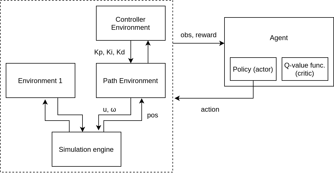
Environment
Environment
Action space:
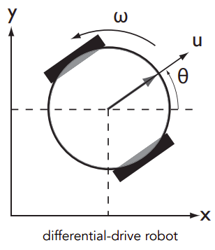
(u, \omega)
Path:
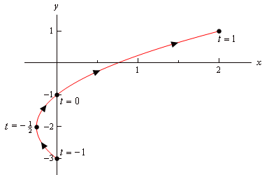
\rho(t)\ \ \text{for}\ t=0\ \text{to}\ 1
Environment
Observation space:
(\rho(t)_{x_r}, \rho(t)_{y_r})
- where t is chosen by the environment as the next point to follow, based on robots position
- coordinates are relative
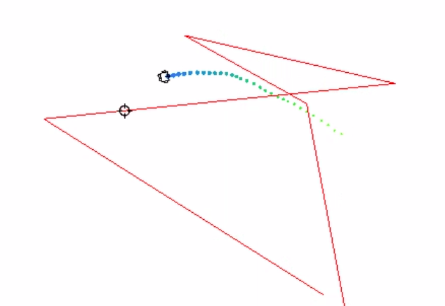
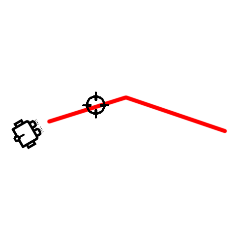
Path handling
- Continuous path randomly generated
- Goals are generated base on the progress
- Robots are trained to head towards goal before handling path following
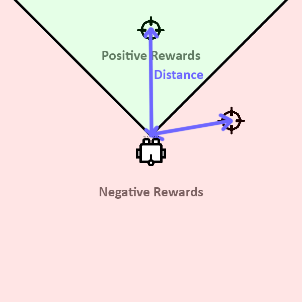
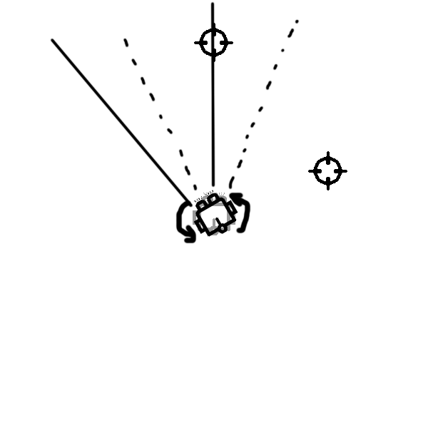
Reward Function
- Direction reward
- Distance reward
- Angular velocity
Total reward = Direction reward + Distance reward - Angular velocity
Reward Function
- Direction reward
- Distance reward
- Angular velocity

Reward Function
- Direction reward
- Distance reward
- Angular velocity
Reward Function
- Direction reward
- Distance reward
- Angular velocity
Extension
Learn hyper-parameters of a feedback-linearized low-level path-following controller
Path-following controller
Move holonomic point
Observation
Agent
(\dot{p_x}, \dot{p_y})
(K_i, K_p, K_d, \epsilon)
controller coefficients
Move holonomic point
- PID coefficients
- Epsilon (holonomic point offset) → feedback linearisation
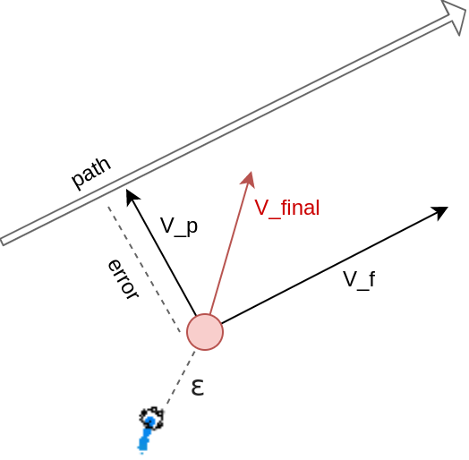
= - \text{PID}(error) * V_p + V_f
(K_i, K_p, K_d)
V_{final} =
(\dot{p_x}, \dot{p_y})
Path-following controller
Move holonomic point
Observation
Agent
(\dot{p_x}, \dot{p_y})
Move the robot
(u, \omega)
(feedback linearization)
Action in the environment
(K_i, K_p, K_d, \epsilon)
controller coefficients
DDPG
Deep Deterministic Policy Gradients
Actor
Policy
Critic
Q-function

Q^*(s_t, a_t) = r_t + \gamma\ \underset{a}{\mathrm{max}}\,Q^*(s_{t+1}, a)
\pi^*(s_t) = \underset{a}{\mathrm{argmax}}\ Q^*(s_t,a)

(\,s_t,\ a_t,\ r_t,\ s_{t+1}\,)
Training [Actor]
Q
\rightarrow \mathrm{max}
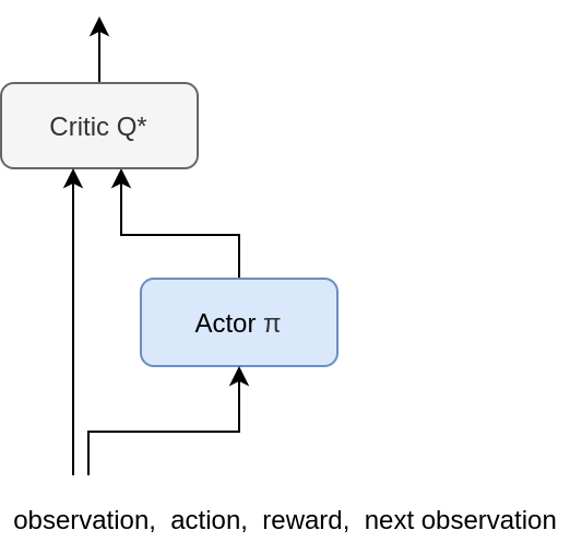
(target)
Training [Critic]
(\,s_t,\ a_t,\ r_t,\ s_{t+1}\,)
Q(s_t, a_t)
= r_t + \gamma\ Q^*(s_{t+1}, \pi^*(s_{t+1}))
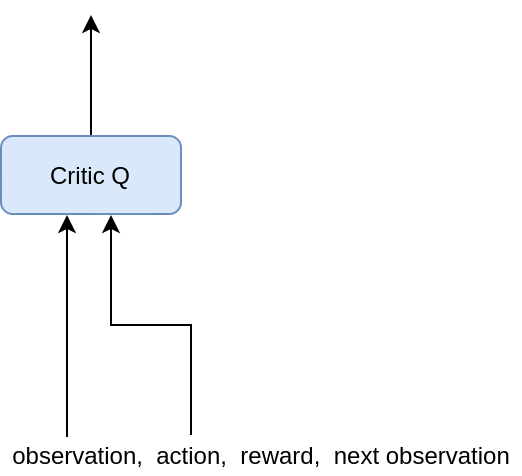
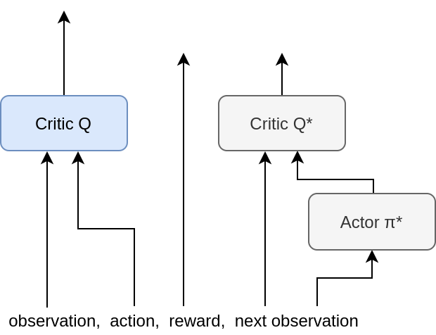
\rightarrow r_t + \gamma\ \underset{a}{\mathrm{max}}\,Q^*(s_{t+1}, a)
(target)
(target)
Updating target networks
- Soft updates:
(polyak averaging)
\theta^Q : \text{Q network}\\
\theta^\pi : \text{policy network}
\theta^{Q^*} : \text{target Q network}
\theta^{\pi^*} : \text{target policy network}
\theta^{Q^*} \leftarrow \tau\theta^Q + (1-\tau)\theta^{Q^*}\\
\theta^{\pi^*} \leftarrow \tau\theta^\pi + (1-\tau)\theta^{\pi^*}
Target networks
Exploration
- Cannot probabilistically select random action
- Add random noise instead
- Ornstein-Uhlenbeck Process
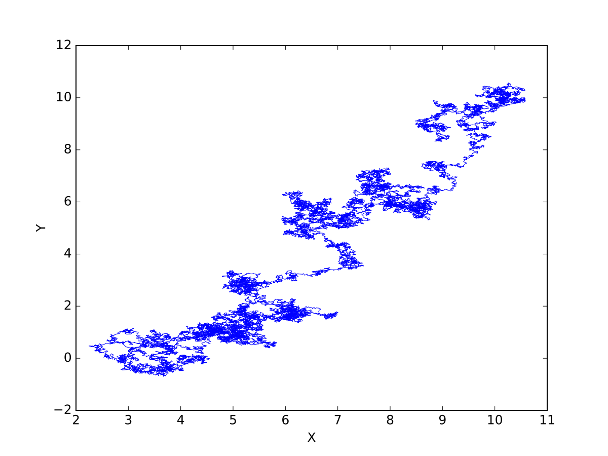
\pi'(s_t) = \pi(s_t) + \mathcal{N}
PPO
Proximal Policy Optimisation
Overview
- Policy Gradient Methods
- Trust Region Policy Optimisation (TRPO)
- Proximal Policy Optimisation (PPO)
Policy Gradient Method
- Increase probability of high reward actions
- Objective Function
L^{\text{PG}} (\theta) = \hat{\mathbb{E}}_t \left[\log \pi_\theta(a_t \vert s_t) \hat{A}_t \right]
- Unstable in practice
- Extremely large policy updates
Advantage Function
Policy Network
Time Step
Action
State
Trust Region Policy Optimisation
- Previously:
- Single bad step can collapse performance
- Dangerous to take large steps!
- Now:
- Constrain size of update
- Still take largest step for improvement
Trust Region Policy Optimisation
- Maximize a surrogate objective
\max_\theta \hat{\mathbb{E}}_t \left[ \frac{\pi_\theta(a_t \vert s_t)}{\pi_{\theta_{\text{old}}}(a_t | s_t)} \hat{A}_t \right]
policy before update
- KL-divergence constraint
\hat{\mathbb{E}}_t \left[\text{KL}[\pi_{\theta_\text{old}}(\cdot \vert s_t), \pi_\theta(\cdot \vert s_t)]\right] \leq \delta
Trust Region Policy Optimisation
- Objective function
- Intuition:
- Take large steps
- New policy cannot be "too different"
- Difference in the form of KL-divergence
\max_\theta \hat{\mathbb{E}}_t \left[ \frac{\pi_\theta(a_t \vert s_t)}{\pi_{\theta_{\text{old}}}(a_t | s_t)} \hat{A}_t - \beta \text{KL}[\pi_{\theta_\text{old}}(\cdot \vert s_t), \pi_\theta(\cdot \vert s_t)] \right]
Scale
Trust Region Policy Optimisation
- Hard to tune beta
- Different problems = different scaling
- Gradient policy update
- Analytical update possible (using natural gradients)
- Expensive 2nd order method to compute
Proximal Policy Optimisation
- Previously:
- Expensive 2nd order method
- Now:
- Use 1st order method
- Use more soft constraints
- Mitigates possible bad decisions
L^{\text{CLIP}}(\theta) = \hat{\mathbb{E}}_t \left[ \min (r_t(\theta)) \hat{A}_t, \text{clip}(r_t(\theta), 1-\epsilon, 1+\epsilon) \hat{A}_t \right]
r_t(\theta) = \frac{\pi_\theta(a_t \vert s_t)}{\pi_{\theta_{\text{old}}}(a_t \vert s_t)}
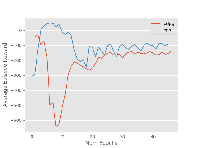
Evaluation
Tools


Algorithms
- DDPG vs PPO
Warmup
Possible extensions
- Expand observation space
- Advanced simulation (Gazebo)
- Obstacles
- Reward: integrate path over a vector field