week 07
Epidemics on networks
Social Network Analysis
Coronavirus COVID-19
Mark Handley, UCL
Coronavirus COVID-19
Mark Handley, UCL
Coronavirus COVID-19
Mark Handley, UCL
Simple model of contagion
Simple model of contagion (decrease transmittion)
- 1st wave: first infected person enters the population and transmits to each person he meets with probibility \( p \). Suppose he meets \( \langle k \rangle \) people while contagious
- 2nd wave: each infected person from 1st wave meets \( \langle k \rangle \) new people and independently transmits infection with probibility \( p \).
- 3nd wave: ...
Galton-Watson branching stochastic process
Branching process
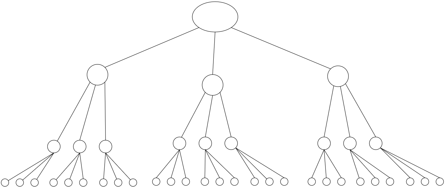
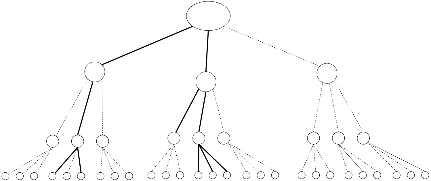
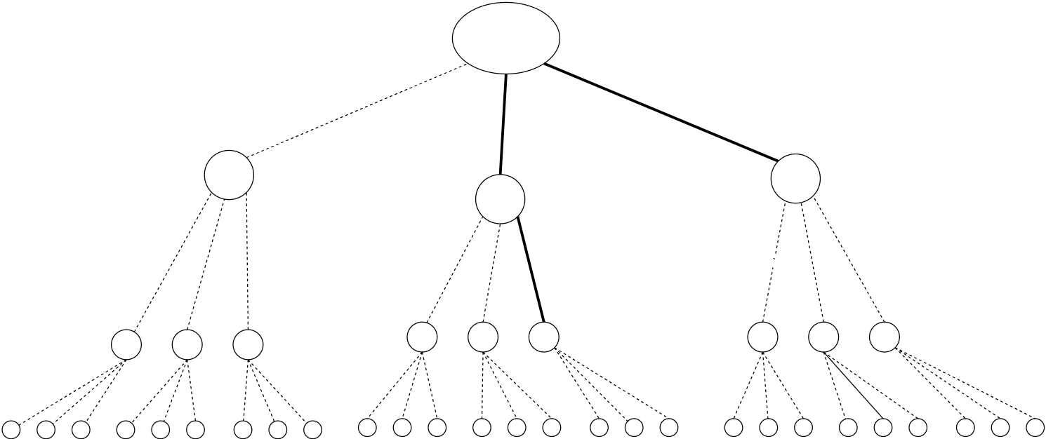
(a)
(b)
(c)
Galton-Watson BP
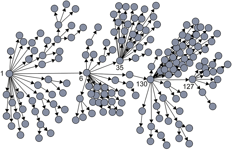
SARS infection in Singapore
Galton-Watson BP
Definition Suppose initially there are \( X_0 \) individuals (the initial generation). In the \( n \) -th generation, the \( X_n \)X individuals independently give rise to numbers of offspring
\( \xi_1^{(n)}, \xi_2^{(n)}, \dots , \xi_{X_n}^{(n)} \), where \( \xi_1^{(n)}, \xi_2^{(n)}, \dots , \xi_{X_n}^{(n)} \) are IID random variable with the same distribution as
The total number produced for the \( (n + 1) \) generation is
Then, Process \( {X_n, n = 0, 1, 2, \dots } \) is a Branching process.
For convenience \( Z_0 = 1 \) is used usually.
An assumption implied in the definition is that \( X_n \) is independent of \( \xi_k^{(m)} \) for all \( k \) and \( m \) .
Branching process
- the average number of new infected nodes/people on every step
- On the rn step, the average number of infected people
- if \(R_0>1 \), the average grows geometrically as \(R_0^n\)
- if \(R_0<1 \), the average shrinks geometrically as \(R_j\)
- when \(n \rightarrow t\), geometric growth \( \rightarrow \) exponential growth
\( R_0 \) - basic reproduction number, is the average number of
secondary infections produced when one infected individual is
introduced into a host population where everyone is susceptible
\( R_0 \) = 1- is the threshold that determines when an infection can
invade and persist in a new host population.
Basic reproductive number
| Disease | Transmission | R0 |
|---|---|---|
| Measles | Airborne | 12-18 |
| Pertussis | Airborne droplet | 12-17 |
| Diptheria | Saliva | 6-7 |
| Smallpox | Social contact | 5-7 |
| Polio | Fecal-oral route | 5-7 |
| Rubella | Airborne droplet | 5-7 |
| Mumps | Airborne droplet | 4-7 |
| HIV/AIDS | Sexual contact | 2-5 |
| SARS | Airborne droplet | 2-5 |
| Influenza (1918 strain) |
Airborne droplet | 2-3 |
Compartmental models in epidimiology
- Mathematical epidemiology
- W. O. Kermack and A. G. McKendrick, 1927
- Deterministic compartmental model (population classes) {S,I,R}
- S(t) - susceptible, number of individuals not yet infected with the disease at time t
- I(t) - infected, number of individuals who have been infected with the disease and are capable of spreading the disease.
- R(t) - recovered, number of individuals who have been
infected and then recovered from the disease, can’t be infected again or to transmit the infection to others.
- Fully-mixing model
- Closed population (no birth, death, migration)
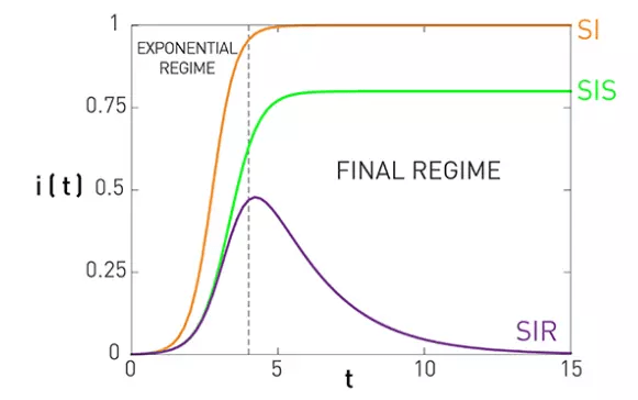
- Models: SI, SIS, SIR, SEIR,
Compartmental models in epidimiology
- \( \beta \)- transmission/infection rate, number of transmitting contacts per unit time; \(T_c=1 \) \( \beta \) - time between transmitting contact
- Infection equation:
SI model
- Fraction:
- Equations
- Differntial equation,
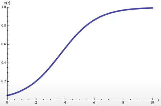
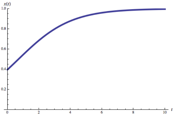
Logistic growth function
- Solution:
- Limit
SIS model
- Infection equations:
- \( \beta \) - infection rate (on contact), \( \gamma \) - recovery rate; \( T_r=1 \) / \( \gamma \) average time to recovery
- Differential equation,
SIS model
- Solution
Where
- Limit \( t \rightarrow \infty \)
Logistic function
Logistic function
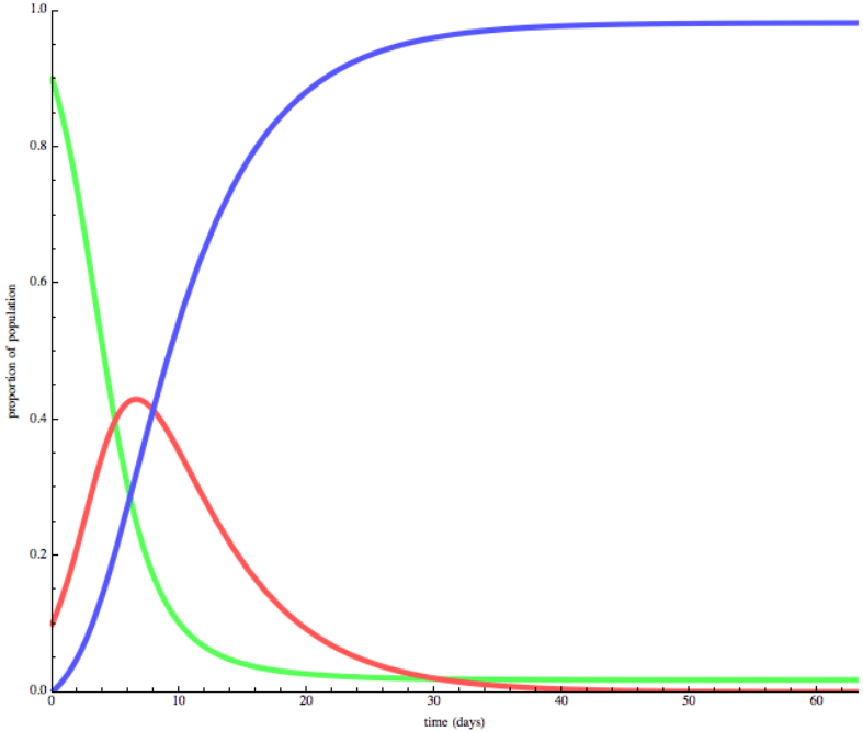
SIR model
- Infection equation:
SIR model
- Solution
- Equation
SIR model
SIR model
SIR model
- Equation
- Limits:
- Initial conditions:
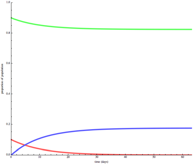
SIR model
SIR model
- \( r_{\infty}\) - the total size of the outbreak
- Epidemic treshold
- \( \beta \) - infection rate, \( \gamma \) - recovery rate \( \rightarrow \)
- Basic reproducnion number
It is average number of people infected by a person before his recovery
SIR model
More models: SIRS and SEIRS
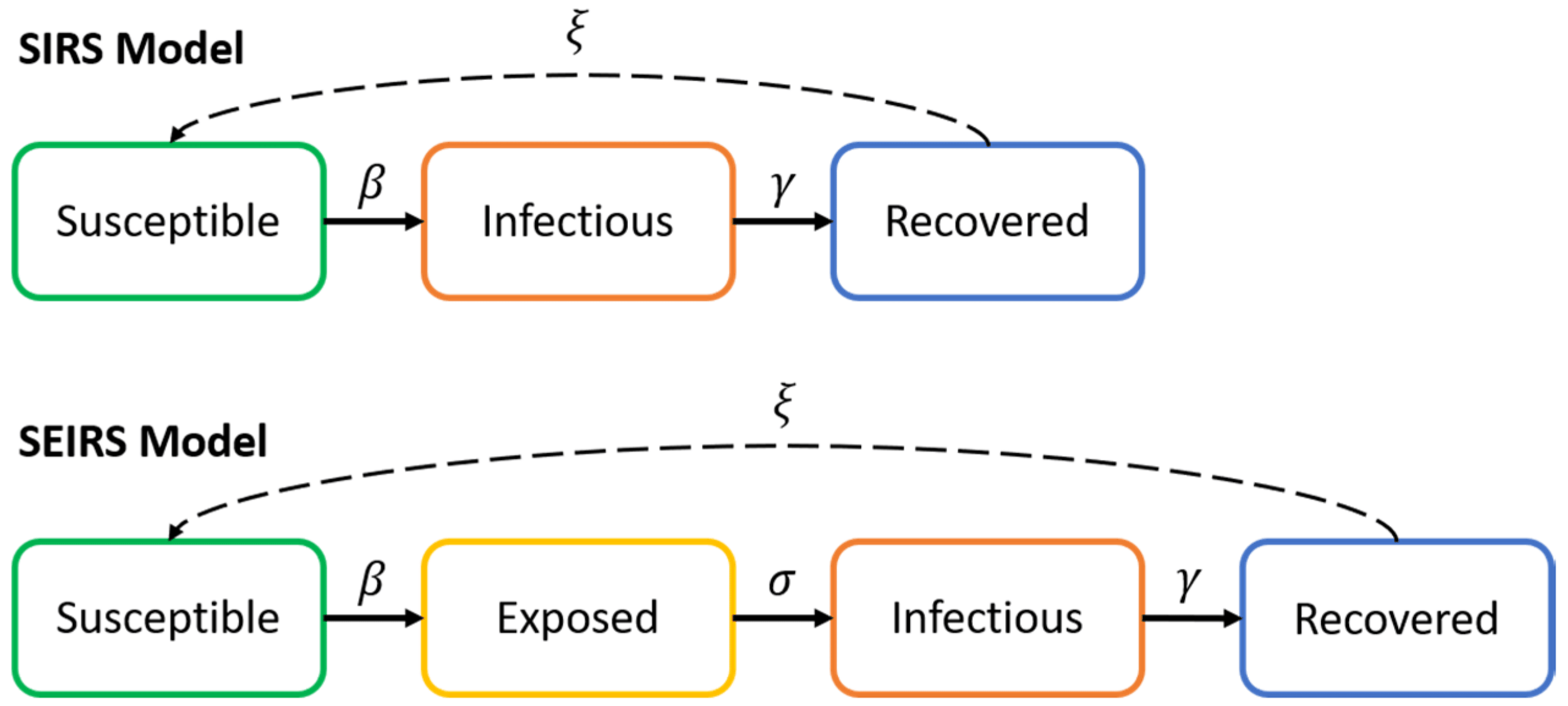
More models: SEIRS-v
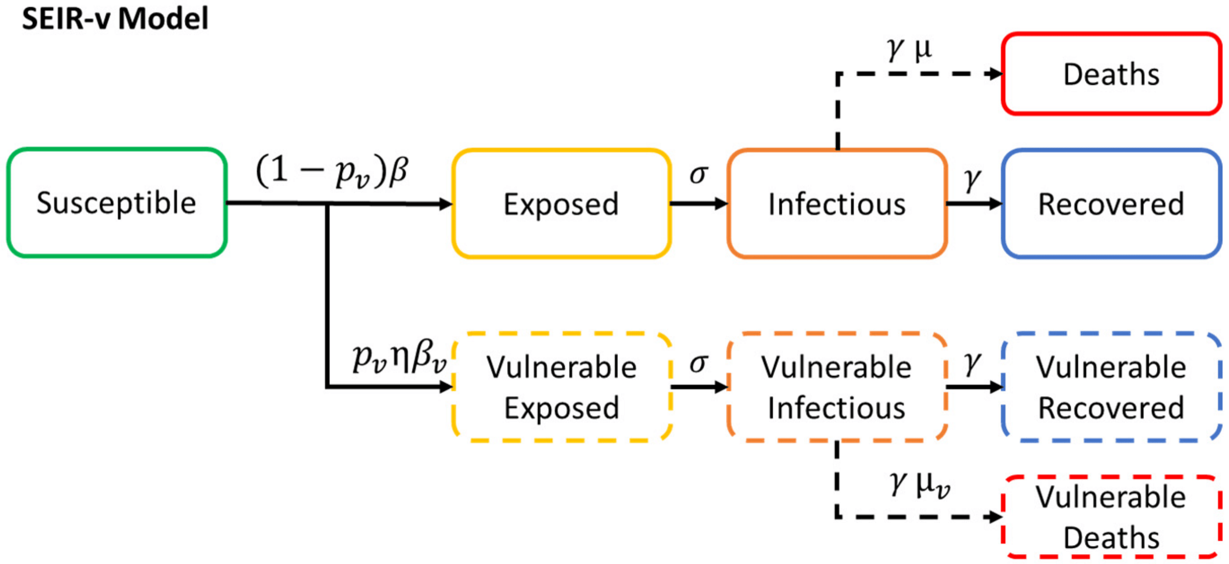
More models: SEIIHURD
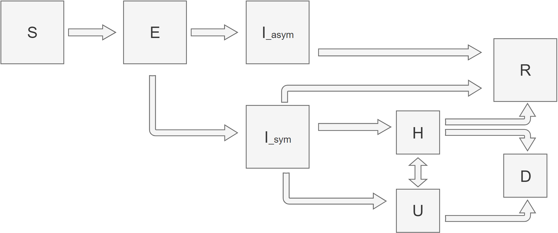
8 - compartamental model:
S - susceptible, E - exposed, I - infectious, H - hospitalised,
U - ICU units, R - recovered
Laplacian Operator
L10
Compartmental models summary
Probabilistic node-level model
- network of potential contacts (adjacency matrix A)
- probabilistic model (state of a node)
\( s_i(t) \) - probabiliti that at \( t \) node \( i \) is susceptible
\( s_i(t) \) - probabiliti that at \( t \) node \( i \) is ifected
\( s_i(t) \) - probabiliti that at \( t \) node \( i \) is recovered
- \( \beta \) - probably that disease will be transmitted on a contact in time \( \delta t \) ( for compartmental model \( \beta_c=\beta\langle k\rangle \)
- \( \gamma \) - recovery rate (probability to recover in a unit time \( \delta t \)
- from deterministic to probabilistic description
- connected component - all nodes reachable
- network is undirected (matrix A is symmetric)
Probabilistic model
Two processes
- Node infection

- Node recovery

SI model
- SI model
- Probabilities that node \( i \): \( s_i (t) \) - susceptible, \( x_i (t) \) - infected at \( t \)
- \( \beta \) - infection rate, probability to get infected in a unit time
- infection equations
SI model
- System of differential equations
- early time approximation, \( t \rightarrow 0, x_i (t) \ll 1 \)
- solution in the basis
SI model
- Solution
- growth rate of infection depends on \( \lambda_1 \)
- probability of infection of nodes depends on \( v_1 \), i.e eigenvector centrality
SI model
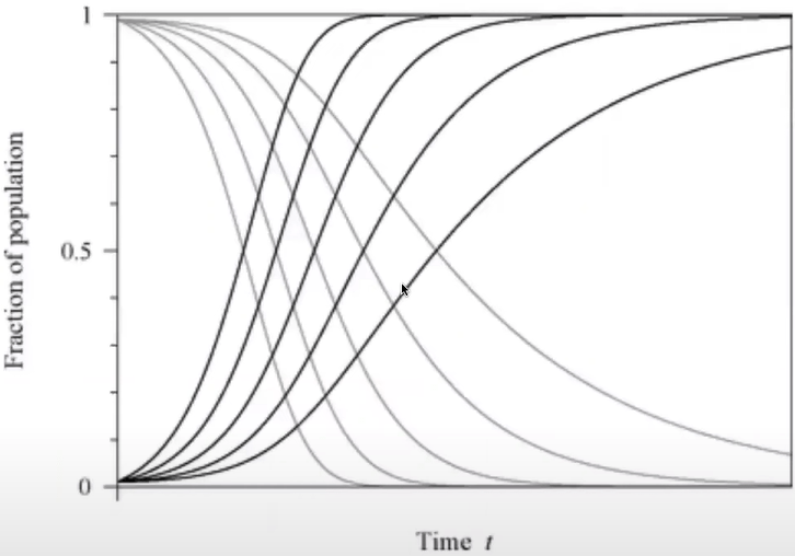
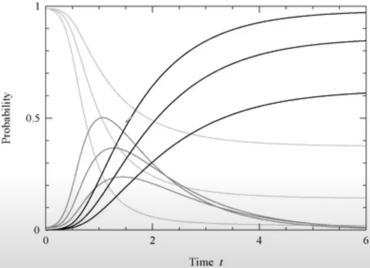
Fractions of susceptible and infected vertices if various degrees in the SI model
The highest values of k the fastest growth
SI model
- Every node at any time step is in one state {S, I}
- Initialize \( c \) in state /
- On each time step each / node has a probability \( \beta \) to infected its nearest neighbors (NN), \( S \rightarrow I \)
Model dynamics :
SI model
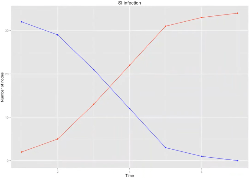
\( \beta \) = 0.5
SIS model
- SIS model
- Probabilites that node \( i \): \( s_i (t) \) - susceptable, \( x_i (t) \) - infected at \( t \)
- \( \beta \) - infection rate, \( \gamma \) - recovery rate
- infection equations:
SIS model
- Differential equation
- early time approximation, \( x_i (t) \ll 1 \)
SIS model
- Eigenvector basis
- Solution
SIS model
- if \( \beta \lambda_1 > \gamma \), infection survives and becomes epidemic
- if \( \beta \lambda_1 < \gamma \), infection dies over time
Epidemic threshold:
- if \( \frac{\beta}{\gamma} > R \), infection survives and becomes epidemic
- if \( \frac{\beta}{\gamma} < R \), infection dies over time
SIS simulation
- Every node at any time step is in one state {S, I}
- Initialise \( c \) nodes /
- Each node stays infected \( \tau_\gamma=\int_0^{\infty} \tau e^{-\tau \gamma} d \tau=1 / \gamma \) time steps
- On each time step each / node has a prabability \( \beta \) to infect its nearest neighbours (NN), \( I \rightarrow S \)
Model dynamics:
SIS model
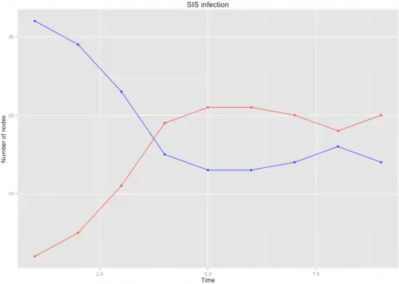
\( \beta \) = 0.5
\( \tau \) = 2
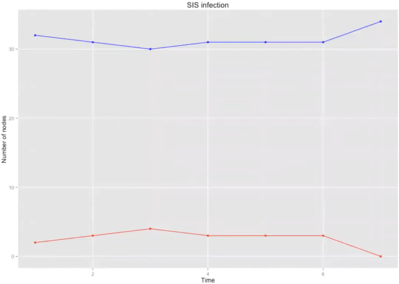
SIS model
\( \beta \) = 0.2
\( \tau \) = 2
SIR model
- SIR model
- Probabilites that node \( i \): \( s_i (t) \) - susceptable, \( x_i (t) \) - infected, \( r_i (t) \) - recovered
- \( \beta \) - infection rate, \( \gamma \) - recovery rate
- infection equations:
SIR model
- Differential equation
- early time,
- Solution
SIR model
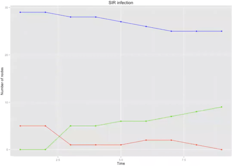
SIR simulation
- Every node at any time step is in one state {S, I, R}
- Initialise \( c \) nodes /
- Each node stays infected \( \tau_\gamma = \frac{1}{\gamma} \) time steps
- On each time step each / node has a prabability \( \beta \) to infect its nearest neighbours (NN), \( S \rightarrow I \)
- After \( \tau_\gamma \) time steps node recovers, \( I \rightarrow R \)
- Nodes \( R \) do not participate in further infection propagation
Model dynamics:
SIR simulation
\( \beta \) = 0.5
\( \tau \) = 2
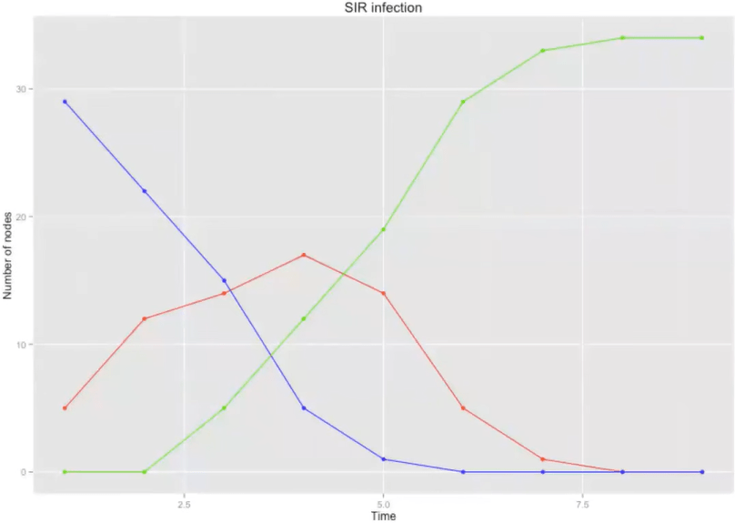
SIR simulation
\( \beta \) = 0.2
\( \tau \) = 2
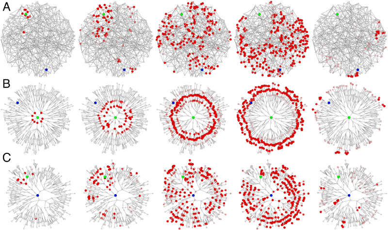
5 Networks, SIR
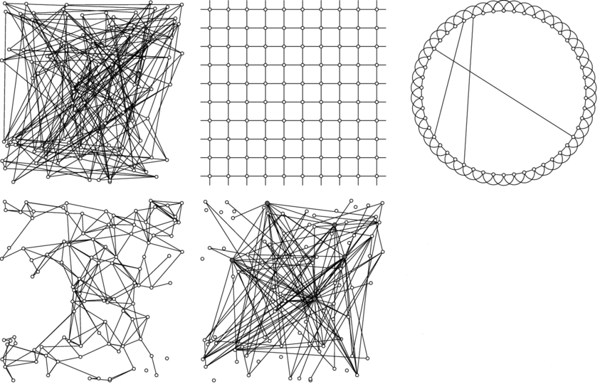
Networks: 1) random, 2) lattice, 3) small world, 4) spatial, 5) scale-free
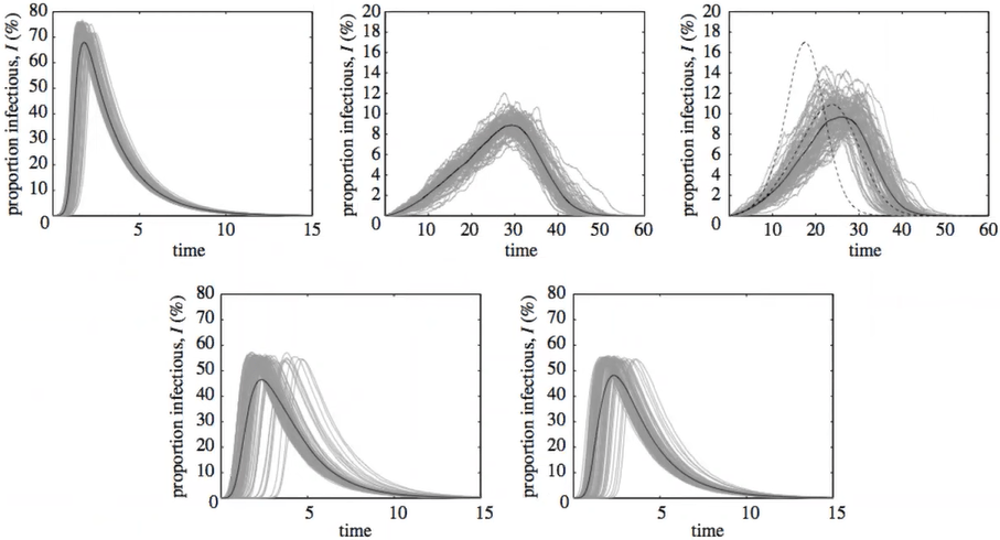
5 Networks, SIR
Networks: 1) random, 2) lattice, 3) small world, 4) spatial, 5) scale-free
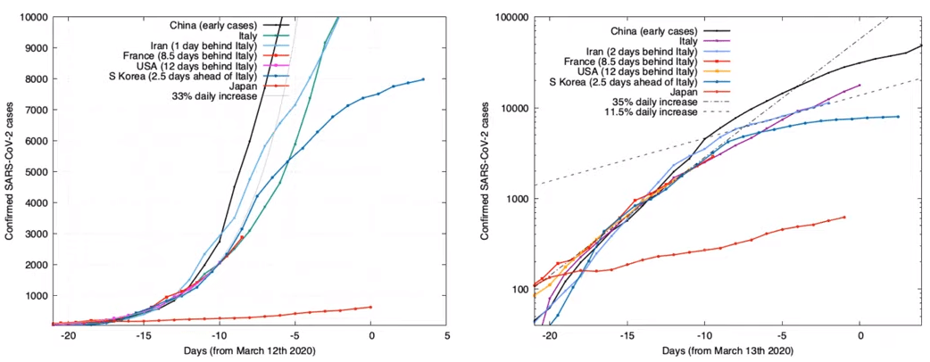
Modeling SARS outbreak
Simulated SIR model: gray lines - passenger flow, red symbols - epidemic location
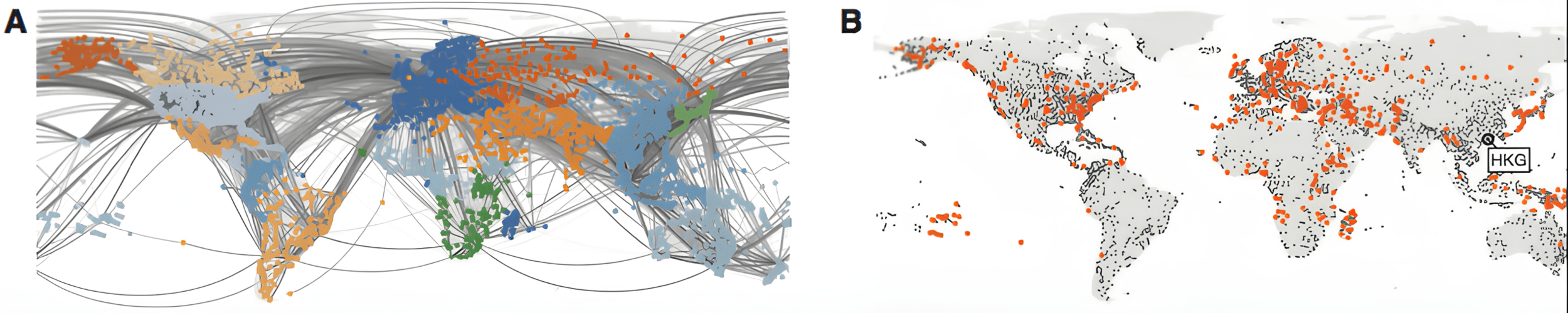
SARS 2003: > 8000 cases, 37 countries
Modeling SARS outbreak
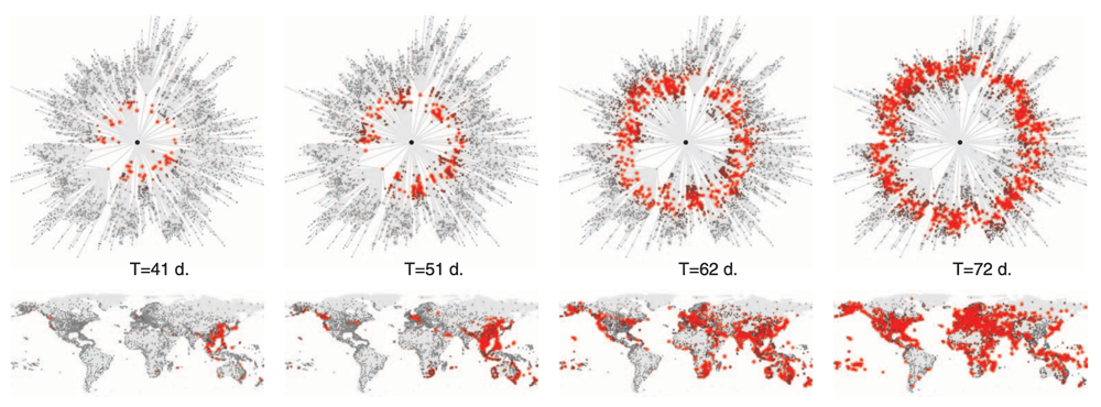
Shortest path three Hong Kong, effective distance
Effective distance
Network synchronization, SIRS
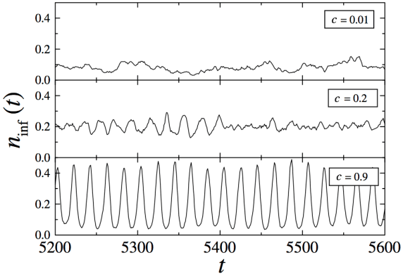
Small-world network at different valyes of disorder parametr \(c\)
Epidemic threshold
One can show that epidemic threshold depends on network homogeneity
- in random network
- in scale-free networks
NO EPIDEMIC THRESHOLD!
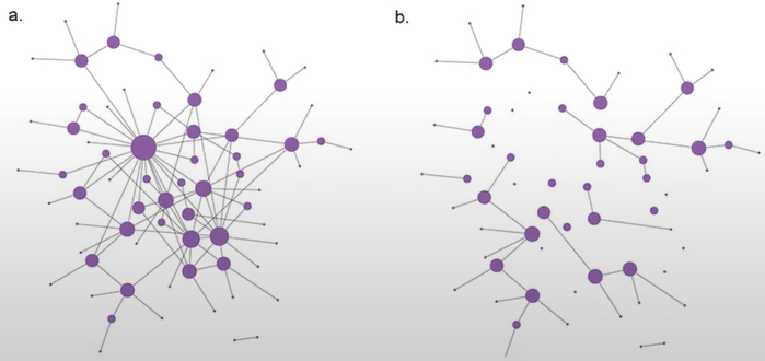
Epidemic threshold
- random vaccination
- hub vaccination \( k > k_{\min} \)
- following random edge \(kP(k) \) degree probability
- random friend vaccination ("friendship paradox")
video ![[whiteboard.png]]
- Competition among memes in a world with limited attention, nature, 2012
- Inf2vec: Latent Representation Model for Social Influence Embedding, IEEE, 2018
- Inf-VAE: A Variational Autoencoder Framework to Integrate Homophily and Influence in Diffusion Prediction, WSDM, 2020
The SIR model wiki
The SIR model is one of the simplest compartmental models, and many models are derivatives of this basic form. The model consists of three compartments:
- S: The number of susceptible individuals. When a susceptible and an infectious individual come into "infectious contact", the susceptible individual contracts the disease and transitions to the infectious compartment.
- I: The number of infectious individuals. These are individuals who have been infected and are capable of infecting susceptible individuals.
- R for the number of removed (and immune) or deceased individuals. These are individuals who have been infected and have either recovered from the disease and entered the removed compartment, or died. It is assumed that the number of deaths is negligible with respect to the total population. This compartment may also be called "recovered" or "resistant".
SIR model takes population, infected cases, recovered cases as input. The model is able to give predictions for an arbitrary time period. As an output, it gives the number of infected and recovery cases.
Model description The SIR model is one of the simplest compartmental models, and many models are derivatives of this basic form. The model consists of three compartments: S for the number of susceptible, I for the number of infectious, and R for the number of recovered or deceased (or immune) individuals. SIR system can be described by the following set of ODE: \( \frac{ds}{dt}= -\frac{βIS}{N} \)
\( \frac{dI}{dt}= \frac{βIS}{N} - \gamma I \)
\( \frac{dR}{dt}= \gamma I \)
where \( \beta \) is the number of people infected at each timestep and \( \gamma \) is the recovery rate. \( S \) is the stock of susceptible population, \( I \) is the stock of infected, \( R \) is the stock of removed population (either by death or recovery), and $N$ is the sum of these three.
The model takes information about the healthy and infected people and simply forecasts the next values based on the ODE system.
Training process Scipy library can be used to calculate ODE’s and fit the SIR parameters (e.g curvefit method in the scipy.optimize module).
Limitations The SIR model does not count many factors and its parameters are considered to be constant. Death predictions The SIR model is not able to predict death cases.
SIR with polynomial contact rate (SIR-poly)
SIR-poly model takes population, infected cases, recovered cases as input. The model is able to give predictions for an arbitrary time period. As an output, it gives the number of infected and recovery cases.
Model description In the basic SIR model we assume a static contact and transition rates through the entire course of the disease, which is not the case for the epidemics. The spread of the disease has led to large changes in societal behavior and so on, which affect the rate of the spread. It is suggested (Conley, 2020) to define the contact rate as a function of active cases. For example, let \( X_i \) be active cases per thousand \( \beta_i \) be the contact rate at a point in time \( i \). \( X_i = \frac{l_i}{N} * 1000 \)
\( \beta_i = \beta_aX_i + \beta_b \)
\( \beta_i \) is then used as a beta in the basic SIR system.
Training process Scipy library can be used to calculate ODE’s and fit the SIR parameters (e.g curvefit method in the scipy.optimize module).
Limitations This model does not count many factors. Death predictions The SIR-poly model is not able to predict death cases.
Influence Models
- Independent Cascade
- \( p_{v,w} \) for each edge
- SI# if \( p_{v,w} = p \)
- Linear Threshold
- \( \sum{w_{ij}} > \theta \)
https://en.wikipedia.org/wiki/Compartmental_models_in_epidemiology
https://publications.hse.ru/en/chapters/210598897
The Hidden Geometry of Complex, Network-Driven Contagion Phenomena
- Epidemics on networks with NetworkX and EoN github
# Information propagation
### Inf2vec: Latent Representation Model for Social Influence Embedding
[ieee](https://ieeexplore.ieee.org/document/8509310), [pdf](https://dl.dropboxusercontent.com/s/hn22yzwdei0lc71/inf2vec.pdf)
The authors propose a model for embedding social influence.
Embedding occurs as follows:
1. For each user, two influence contexts are defined: local and global. Local context is a set of users obtained using random-walk via propagation network, global context is a set of users similar in their actions.
2. Embedding consists of two parts (two vectors): -
1. Source Embedding - responsible for the user’s ability to influence others (S)
2. Target Embedding - responsible for how much the user is influenced (T)
3. biases - influenceability and conformity
3. Based on contexts and chains of actions for pairs of users, the probabilities of influence of one user on another are calculated, the probability is calculated through a combination of S, T, biases, thus the vectors are fit.
[feng2018.pdf](https://s3-us-west-2.amazonaws.com/secure.notion-static.com/65ba9b1f-cf93-438e-9fa4-cc7bb7a87103/feng2018.pdf)
Inf2Vec model improvement + Influence Maximization task
Applying the model from the previous article to the problem of maximizing influence.
In principle, the authors do not make changes to the model, they only discover that for their task it is enough to look only at users who mainly start activities, they also simplify the calculations (as far as I understand, they make a lightweight model in which embeddings are not calculated)
[7319-Article Text-10549-1-10-20200601.pdf](https://s3-us-west-2.amazonaws.com/secure.notion-static.com/a8e0649e-4ca4-4d63-b7fe-645ed4849fc3 /7319-Article_Text-10549-1-10-20200601.pdf)
Deep Collaborative Embedding (DCE)
Autoencoder of information propagation cascades. First, cascading contexts are collected there, which for each cascade make an N*N matrix (N is the number of nodes), where the values on [i, j] are the potential influence of user i on user j within this cascade.
Then, for each node, the vectors of their influence on other nodes within different cascades are collected, and all this is fed to the input of the autoancoder, from which the embedding for the node is obtained.
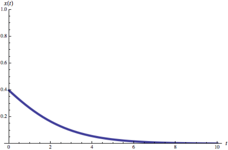
Susceptible-Infected-Susceptible (SIS) Model
Most pathogens are eventually defeated by the immune system or by treatment. To capture this fact we need to allow the infected individuals to recover, ceasing to spread the disease. With that we arrive at the so-called SIS model, which has the same two states as the SI model, susceptible and infected. The difference is that now infected individuals recover at a fixed rate μ, becoming susceptible again. The equation describing the dynamics of this model (2) is an extension of (1)
(1)
(2)
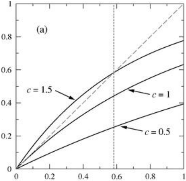
where μ is the recovery rate and the μi term captures the rate at which the population recovers from the disease. The solution of (2) provides the fraction of infected individuals in function of time
Disease-free State (μ > β〈k〉)
For a sufficiently high recovery rate the exponent in (3) is negative. Therefore, i decreases exponentially with time, indicating that an initial infection will die out exponentially. This is because in this state the number of individuals cured per unit time exceeds the number of newly infected individuals. Therefore with time the pathogen disappears from the population.
(3)
where the initial condition
In other words, the SIS model predicts that some pathogens will persist in the population while others die out shortly. To understand what governs the difference between these two outcomes we write the characteristic time of a pathogen as
(4)
where
(5)
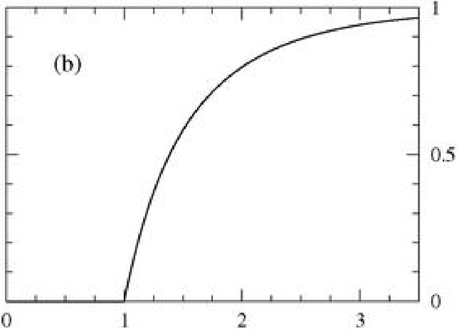
The Basic Reproductive Number, R0
\(R_0\) is the basic reproductive number. It represents the average number of susceptible individuals infected by an infected individual during its infectious period in a fully susceptible population. In other words, \(R_0\) is the number of new infections each infected individual causes under ideal circumstances. The basic reproductive number is valuable for its predictive power:
- If \(R_0\) exceeds unity, τ is positive, hence the epidemic is in the endemic state. Indeed, if each infected individual infects more than one healthy person, the pathogen is poised to spread and persist in the population. The higher is \(R_0\), the faster is the spreading process.
- If \( R_0 < 1 \) then τ is negative and the epidemic dies out. Indeed, if each infected individual infects less than one additional person, the pathogen cannot persist in the population.
The Basic Reproductive Number, R0
The reproductive number (5) provides the number of individuals an infectious individual infects if all its contacts are susceptible. For \( R_0 < 1 \) the pathogen naturally dies out, as the number of recovered individuals exceeds the number of new infections. If \( R_0 > 1 \) the pathogen will spread and persist in the population. The higher is \( R_0 \), the faster is the spreading process. The table lists \( R_0 \) for several wellknown pathogens.
Consequently, the reproductive number is one of the first parameters epidemiologists estimate for a new pathogen, gauging the severity of the problem they face. For several well-studies pathogens \( R_0 \) is listed in Table. The high \( R_0 \) of some of these pathogens underlies the dangers they pose: For example each individual infected with measles causes over a dozen subsequent infections