week 04
Clustering and Community Detection
Social Network Analysis
03-2
Community Detection General Idea
Connected and undirected graphs
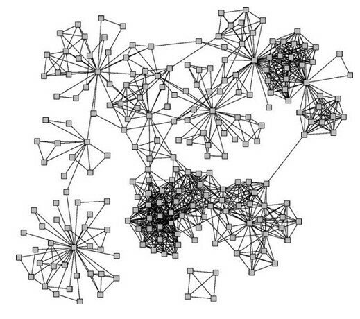
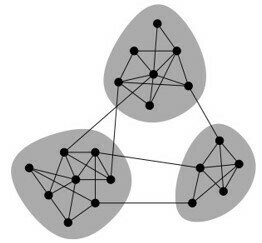
Network Communities
What makes a community (cohesive subgroup):
- Mutuality of ties. Everyone in the group has ties (edges) to one another
- Compactness. Closeness or reachability of group members in small number of steps, not necessarily adjacency
- Density of edges. High frequency of ties within the group
- Separation. Higher frequency of ties among group members compared to non-members
Wasserman and Faust
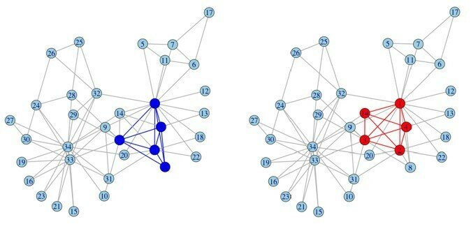
Graph cliques
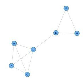
A clique is a complete (fully connected) subgraph, i.e. a set of vertices where each pair of vertices is connected.
Cliques can overlap
Graph cliques
- A maximal clique is a clique that cannot be extended by including one more adjacent vertex (not included in larger one)
- A maximum clique is a clique of the largest possible size in a given graph
- Graph clique number is the size of the maximum clique
Graph cliques
Maximum cliques
Maximal cliques:
Clique size: 2 3 4 5
Number of cliques: 11 21 2 2
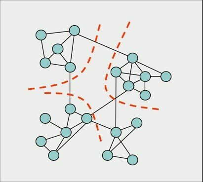
Network comminities
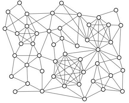
Network communities are groups of vertices such that vertices inside the group connected with many more edges than between groups.
Community detection is an assignment of vertices to communities. Will consider non-overlapping communities, graph cuts
Community detection
Consider only sparse graphs m «n2 Each community should be connected Combinatorial optimization problem:
- optimization criterion (cut, conductance, modularity)
- optimization method
Exact solution NP - hard
(bi-partition: n = n1 + n2, n!/(n1!n2!) combinations)
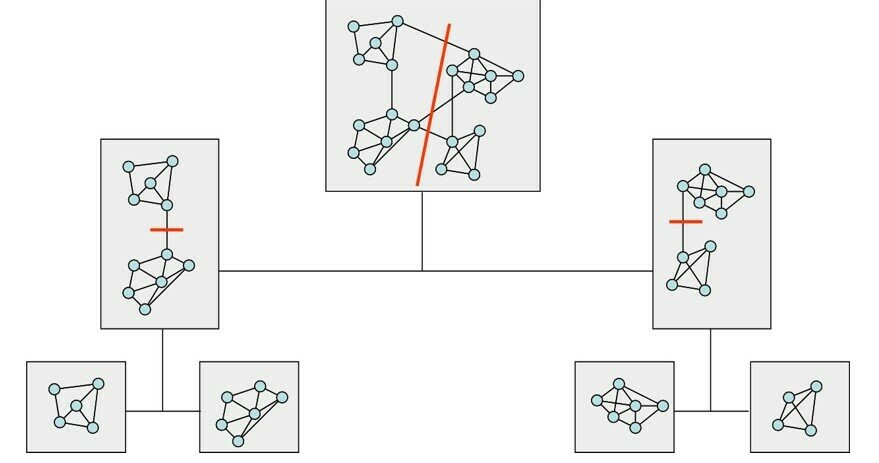
Solved by greedy, approximate algorithms or heuristics. Recursive top-down 2-way partition, multiway partition. Balanced class partition vs communities
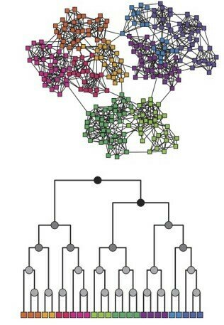
recursive partitioning
Edge betweenness
Focus on edges that connect communities.
Edge betweenness - number of shortest paths σst (e) going through edge e
Construct communities by progressively removing edges
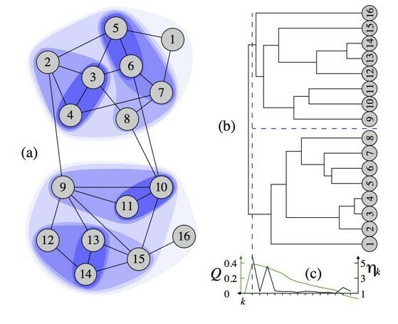
Edge betweenness algorithm
Newman-Girvan, 2004
Algorithm: Edge Betweenness
Input: graph G(V,E)
Output: Dendrogram/communities
Repeat
For all e ∈ E compute edge betweenness CB (e);
remove edge ei with largest CB (ei ) ;
until edges left;
If bi-partition, then stop whrn graph splits in two components (check for connectedness)
Hierarchical algorithm, dendrogram
03-3
Community Detection Quality
- Various goodness metrics that evaluate structural properties of communities.
- Density - fraction of internal edges out of total number of possible edges.
- Conductance - fraction of total edge volume that points outside the cluster.
- Modularity - the difference of the number of edges in a community and the expected number of edges (assuming you have an identical degree distribution).
Community Detection Metrics
Fortunato, Newman, 20 years of network community detection, Nature Physics, 2022, [pdf]
Metric: Density
Example:
Metric: Conductance
Example:
Measure of internal and external connectivity. The fraction of edges pointing outside a community
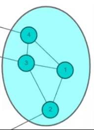
Metric: Modularity
- A global metriic: defined per-network, not per-community
- Measure of internal and external connectivity. How well network partitions into modules
- Higher values are better
normalize by degree sum
sum goes through every pair of verticies
Kronecker delta function == 1 only if u and v are in the same community
Metric: Modularity
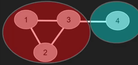
| v=1 | v=2 | v=3 | v=4 | |
|---|---|---|---|---|
| u = 1 | (0 - (2*2)/8)*1 | (1 - (2*2)/8)*1 | (0 - (2*1)/8)*0 | |
| u = 2 | (1 - (2*2)/8)*1 | (0 - (2*2)/8)*1 | (1 - (2*3)/8)*1 | (0 - (2*1)/8)*0 |
| u = 3 | (1 - (3*2)/8)*1 | (0 - (3*3)/8)*1 | ||
| u = 4 | (0 - (1*2)/8)*0 | (0 - (1*2)/8)*0 | (0 - (1*1)/8)*1 |
Q = 1/8 * (...+...+...)=-0.031
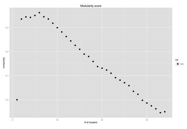
Modularity - Values
- Modularity bounded in range [-0.5, 1]
- All nodes in a single community or all nodes in their own community \( \rightarrow Q=0 \)
- Nonzero values represent deviations from randomness (for better or worse)
- values > 0.3 is an indicator of good community structure
Modularity - Another Equation
Modularity: Directed and Weighted
Weighted:
Directed:
- \( o \) - outgoing edges
- \( i \) - ingoing
Modularity score
03-4
Modularity Maximization Heuristics
Modularity Maximization Heuristics
- Edge Motif (EdMot) (Li, 2019)
- Leiden (Traag, 2019)
- Paris (Bonald, 2018)
- Belief (Zhang & Moore, 2014)
- Combo (Sobolevsky, 2014)
- Leicht-Newman (LN) (Newman, 2008)
- Louvain (Blondel, 2008)
- Greedy (CNM) (Clauset, 2004)
- Graph Neural Network (Sobolevsky, 2022)
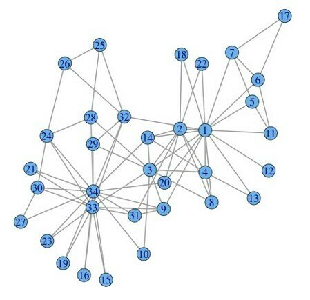
Input
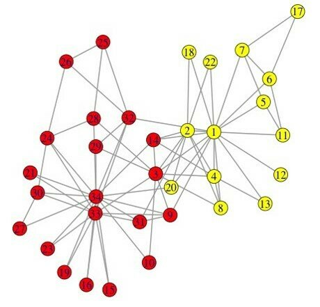
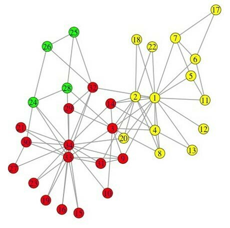
Desired
output
Spectral modularity maximization
- Algorithm: Spectral modularity maximization: two-way partition
- Input: adjacency matrix \( A \)
- solve for maximal eigenvector \( Bx = \lambda x \) ;
- set \( s= sign(x )_{max} \)
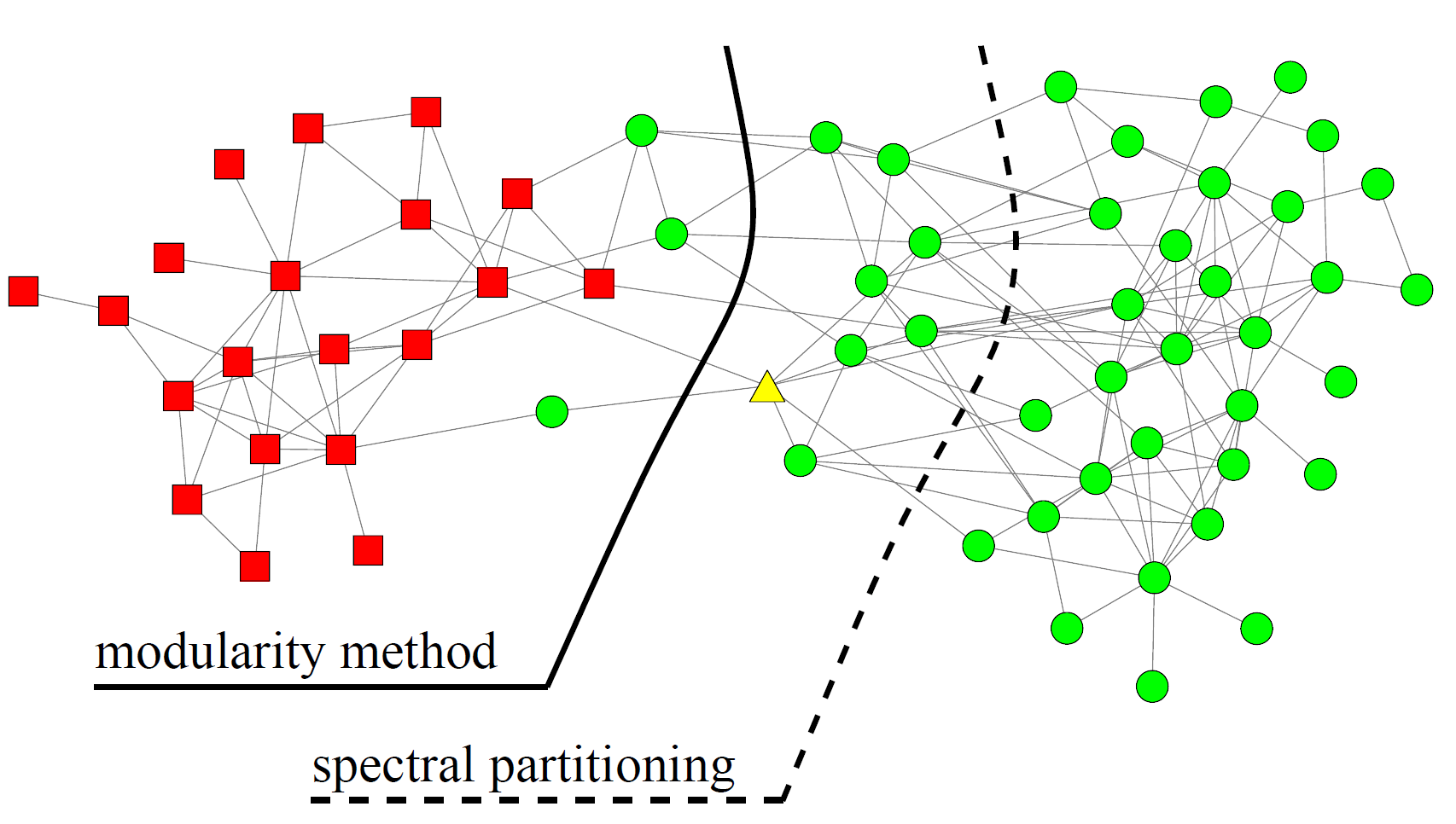
clusters = 5, modularity = 0.437

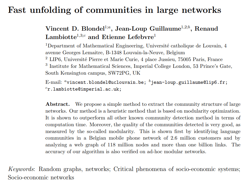
The Louvain method
- Heuristic method for greedy modularity optimization
- Find partitions with high modularity
- Multi-level (multi-resolution) hierarchical scheme
- Scalable
Blondel, Fast unfolding of communities in large networks, 2008
The Louvain method: 1st phase
- Put each node in a graph into a distinct community (one node per community)
- For each node \( i \), the algorithm performs two calculations:
- compute the modularity delta \( (\Delta Q) \) when putting node \( i \) into the community of some other neighbour \( j \)
- Move \( i \) to a community of node \( j \) that yelds the largest gain in \( \Delta Q \)
Fast community unfolding algoritm
Algorithm: Fast unfolding
Input: Graph \( G(V,E) \)
Output: Communities
Assign every node to is own community:
repeat
repeat
until no more improvement (local max of modularity):
Nodes from communities merged into "super nodes":
Weight on the links added up
until no more changes (max modularity):
For every node evaluate the modularity delta \( (\Delta Q) \) when putting node \( i \) into the community of some other neighbour \( j \);
Move \( i \) to a community of node \( j \) that yelds the largest gain in \( \Delta Q \).
Phase 1: Partitioning
Removing \( i \) from \( D \)
Merging \( i \) into \( C \)
Before
Intermediate
After
\( D - i \)
\( D - i \)
\( C + i \)
\( C \)
\( D \)
\( C \)
\( i \)
\( i \)
\( i \)
Phase 2: Summary
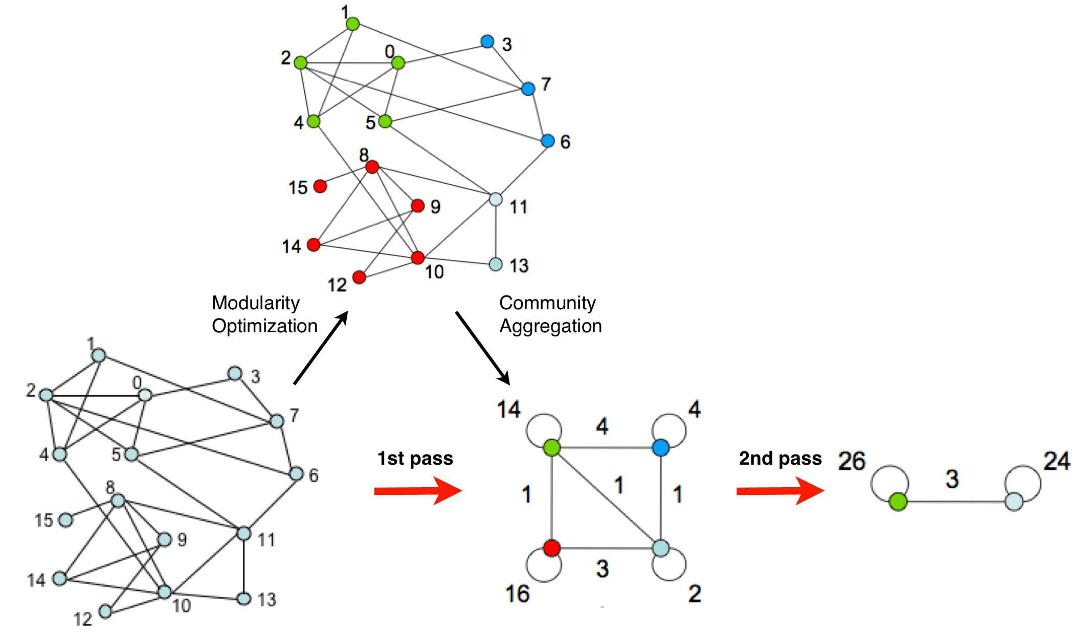
Each pass is made of two phases:
- one where modularity is optimized by allowing only local changes of communities;
- one where the found communities are aggregated in order to build a new network of communities. The passes are repeated iteratively until no increase of modularity is possible.
best: clusters = 6, modularity = 0.345
03-5
Exact/Approximate Modularity Maximization
Exact/Approximate Modularity Maximization
- Integer Programming - IP (Brandes, 2007)
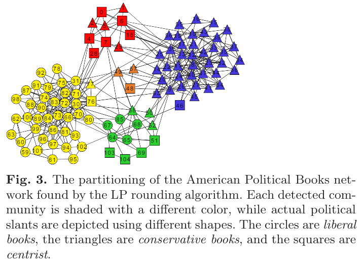
- IP and LP rounding (Agarwal 2008)
- Column generation (Aloise, 2010)
- Sparse IP and LP rounding (Dinh, 2015)
- Approximation (Kawase, 2021)
- Bayan algorithm (Aref, 2022)
Input
Desired
output
Modularity-Maximizing Graph Communities via Mathematical Programming
Bayan algorithm
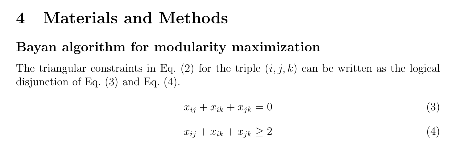
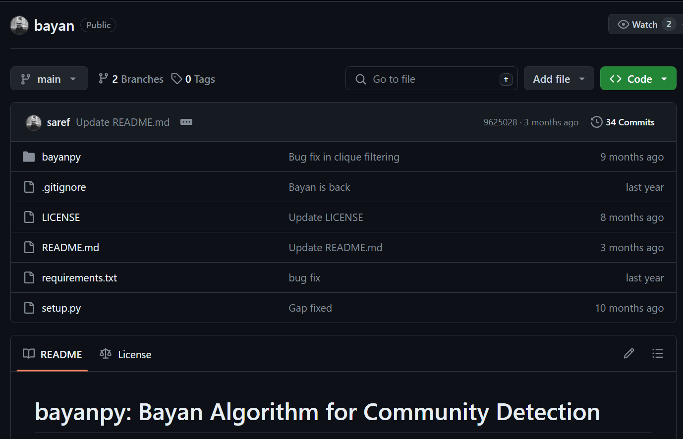
https://github.com/saref/bayan
03-6
Other Community Detection Algorithms
Other Methods
- Kernigan-Lin bisection (Kernigan and Lin 1970)
- RB Potts model with
- Chinese whispers
- Walktrap
- k-cut
- Asynchronous label propagation
- Infomap
- Genetic Algorithm
- Semi-synchronous Label propagation
- Constant Potts Model (CPM)
Other Methods
- Significant scales
- Stochastic Block Model SBm)
- SBM with Monte Carlo Markov Chain
- WCC
- Surprise
- Diffusion Entropy Reducer
- GemSec
- Bayesian Planted Partition
- Markov Stability
Input
Desired
output
Label propagation algorithm
Input: Graph G (V,E)
Output: Communities
Initialize labels on all nodes:
Randomized node order:
repeat
For every node replace its label with occurring with the highest
frequency among neighbors (ties are broken uniformly randomly);
until every node has a label that the maximum number of the neighbors have;
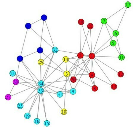
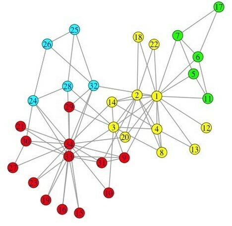
clusters = 3, modularity = 0.435
clusters = 4, modularity = 0.445
Walktrap
Algorithm: Walktrap community detection
Input: Graph G(V,E)
Output: Dendrogram/communities
Assign each vertex to its own community:
Compute random walk distance between adjacent vertices:
for n-1 steps do
choose two "closest" communities and merge them:
update distance between communities
ens
P. Pons and M. Latapy, 2006
clusters = 4, modularity = 0.440
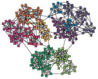
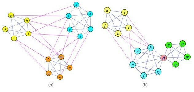
Community detection:
Graph partitioning(sparse cuts)
Vertex clustering (vertex similarity)
image from W. Liu , 2014
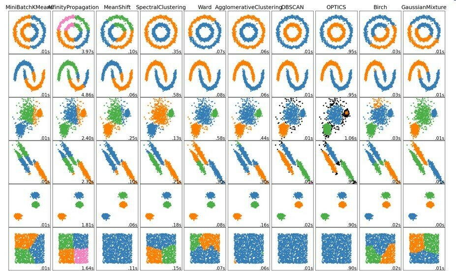
Clustering methods
Takeaway
-
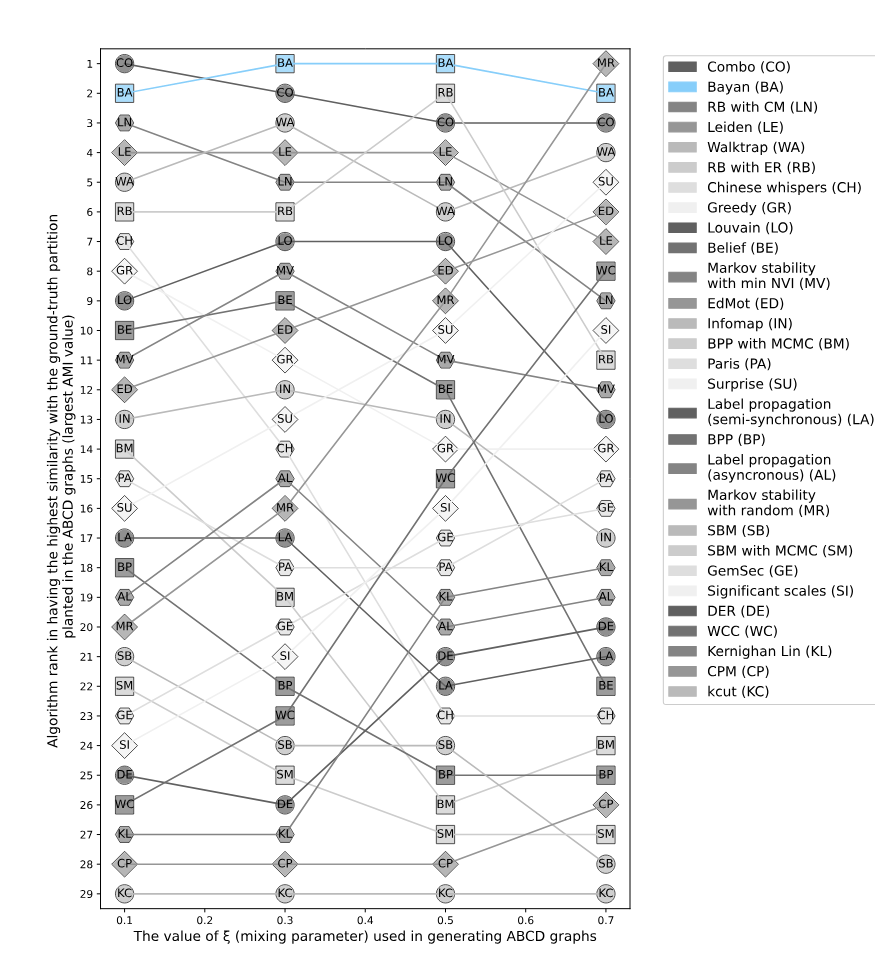
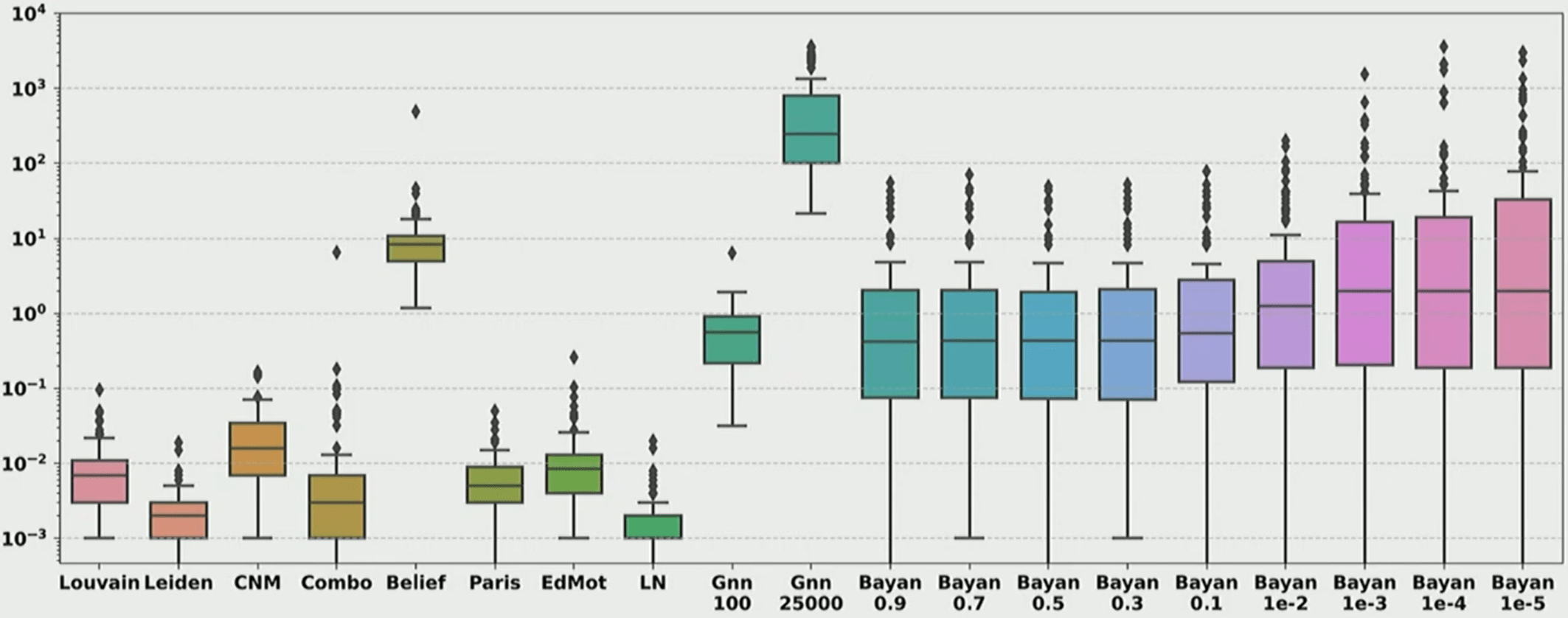
Heuristic modularity maximization algorithms rarely maximize modularity
- Only 19.4%-43.9% of the times on synthetic and real networks
- Suboptimal partitions of heuristic algorithms are disproportionately dissimilar to any optimal partition
Temporal community Detection
- Global:
- Community Detection from scratch and match
- Dependent or Temporal Trade - off Community Detection
- Simultaneous or Offline Community Detection
- Online Community Detection in fully Temporal Networks and in growing Temporal Networks
- Local: Community Detection in Temporal Networks using Seed Nodes
References
Contest 1
3 prizewinners:
- first 10
- second, third 9
- Modularity > strong baseline (0.657) = 8
- Modularity > weak baseline (0.65) = 6
- Any solution = 4
- 5 final submissions.
- All submission's are supposed to be supported with code.
- The code should reproduce declared Modularity in 6/10 starts with different random seeds.