week 12
RecSys
Social Network Analysis
GNN Problems
Observation: more layers = worse performance
Paradoxically, need more layers to capture long-range information
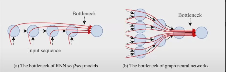
The number of layers needs to match the Bottleneck of Graph Neural Networks, which conceptualizes the distance away from a node that contains information important to the task.
Adding layers often gives exponential increase in receptive field (i.e., you get the neighbors’ neighbors) – lots of information to capture since we need the neighbors of the neighbors of the neighbors.
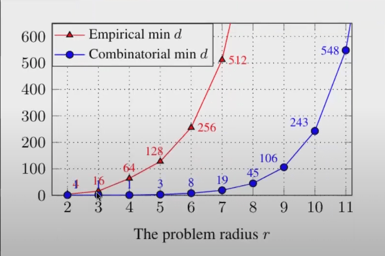
Given a d-dimensional vector of 32-bit float values flatten each float into 32-digit binary vector to represent states: Ω=232d This gives an upper-bound on the number of structures a vector could possibly distinguish among. Capacity needed to fit training data of a toy problem:
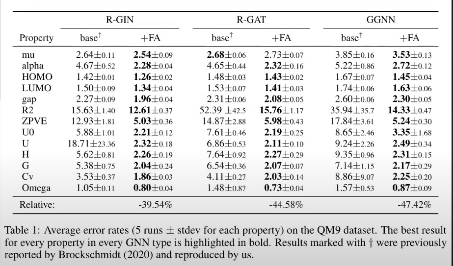
Adding fully-connected adjacency (“FA”) layers for final GNN layer (i.e., pretended graph was fully connected) consistently improved performance
This shows that there was meaningful info in other nodes that wasn’t captured by the multi-layered GNN
However, using FAs in all layers (i.e., ignoring real graph structure) produced much worse results
Best improvement achieved for GGNN's
Over-smoothing vs Over-squashing
Over-smoothing: node representations become indistinguishable when the number of layers increases due to taking aggregates of aggregates of…
Over-squashing: information from an exponentially-growing receptive field is compressed into fixed-length node vectors
Similar in concept to RNNs, which need to represent e.g., a sequence of words in a fixed-length vector, and this can become a bottleneck for long sequences
Solution 1: Skip Connections
High-level idea: copy/paste information from a lower layer so that the new layer doesn’t have to keep track of everything • Several different types…
Residual connection—connect l−1 to l: ℎ^l=f(ℎl,ℎl−1)
Initial connection—connect l=0 to all l: ℎ^l=f(ℎl,ℎ0)
Dense skip connection—connect l′<l to l: ℎ^l=f(ℎl,ℎl′|l′<l)
Jumping Knowledge connection—connect all layers to the final layer: ℎ^L=f(ℎL,ℎl|l<L)
Solution 2: Graph Normalization
High-level idea: ”re-scale node embeddings over an input graph to constraint pairwise node distance and thus alleviate over-smoothing” Bag of Tricks for Training Deeper Graph Neural Networks A Comprehensive Benchmark Study
Several different types…
Batch Normalization: normalize based on statistics of the minibatch
PairNorm: maintain consistent pairwise distance among nodes
NodeNorm: normalize each node separately based on feature variation
Other tricks
Solution 3: Graph Rewiring
High-level idea : change the graph (edge set) to make it more message-passing friendly
There is no guarantee that the natural graph structure is equal to the one that expresses optimal computational dependencies
There are noisy edges, and some important relationships may not be captured by an edge
Diffusion-based approaches: smooth A with a diffusion process (includes multi-hop info) and sparsify to get a new A
Geometric “Ricci-curvature” approach: selectively remove edges that bridge different communities, as this causes the exponential increase
Improving Scability
Sampling
Many real-world/industrial graphs are billions of nodes and edges, perhaps 100s of billions
E.g., E-commerce products, reviews, transactions, sign-in events
You may not even be able to fit this into memory In small-world graphs like social networks, ~6 GNN layers means every node in the graph is needed to calculate each node embedding.
We don’t need the full graph to compute useful embeddings
In fact, having this source of randomness may make your model generalize betterto new, slightly different neighborhoods
We can sample at different levels:
Subset of neighbors of each node during message passing
A set of nodes for each GNN layer
A subset of the graph for the full GNN
Node-level Sampling
Random neighbor sampling: for each node, only choose a subset of neighbors for message passing (e.g., GraphSage).
Still suffers from exponential growth with layers, but controllable
Importance sampling: try to improve the variance of your estimate by smarter sampling
FastGCN and LADIES use importance sampling at the layer-level to reduce exponential growth to linear growth
Subgraph sampling
Cluster-GCN: Find densely connected clusters and only sample neighbors in the same cluster
GraphSAINT : Create random subgraphs for each minibatch and model with a GCN as if it were the full graph
Pre-computation
Idea: instead of doing message passing before each MLP layer, do graph-based processing once
Assumes that the non-linearity between GNN layers is not important, so the model fitting phase is ~ logistic regression
Can be done in one big batch-processing job, not during training process
Simple Graph Convolution (SGC): H=softmax(AKXθ)
Scalable Inception Graph Neural Networks (SIGN): Similar to SGC, but also consider general operators, not just powers of A (e.g., counting triangles, diffusion operators like Personalized Page Rank,..., etc) and concatenate results as features
Resource management
There are optimizations that can be made to improve resource utilization
GNNAutoScale caches historical embeddings from previous minibatches to avoid re-computing them
ROC and DistGNN enable fast/scalable distributed training via memory and graph partitioning optimizations
Graph Classification and Regression Overview
Examples
Predict if this molecule:
- Is toxic
- Activates a protein / Treats a disease
- General properties of molecules
Predict the biological taxonomy of a protein interaction network
What type of object a point cloud represents
The expression made by a face, represented as a mesh
Overall Architecture
Input features X for nodes and edges, when available
OPTIONAL: Preprocess features by passing through an MLP, shared across the nodes
Stack GNN layers to incorporate graph neighborhood information and get node embeddings
Use a Readout function to pool node-level embeddings into a graph-level embedding
Use the graph-level embedding to make a prediction (e.g., with an MLP) on the graph
Loss functions are the standards: cross-entropy for classification tasks, mean-squared error for regression
Graph Pooling with Set Pooling
Set pooling: map a set of embeddings to a single embedding
Does not consider graph topology
Sets do not have a natural order and the operation should therefore be Permutation Invariant
Can use the same Permutation Invariant functions we used when creating node-neighborhood representations in GNNs: aggregation functions like SUM, MEAN, MAX, …, etc.
E.g., hG=∑i∈Vhi
Graph Pooling with Coarsening
Graph coarsening: hierarchically cluster using graph structure
-
Iteratively down-samples, typically by clustering nodes and representing the cluster by a single embedding
-
For each iteration, the adjacency matrix is changing.
-
-
Clustering operation needs to be differentiable so operation can be used end-to-end
-
E.g. Graph U-Nets, which projects nodes into 1-dimension using learnable linear layer and chooses k-largest ones as subset for next iteration.
-
Nuances of Graph Batching
In previous tasks, we had one large graph and were sampling nodes and their k-hop neighborhoods
Now: 1 sample = 1 full graph, no edges between graphs in the batch
How should we do message passing?
Could loop over each graph and run MP separately (slow)
The batched “super-graph”
Alternatively, could create a “super-graph” that creates a block-diagonal adjacency matrix of disconnected components and run MP once (fast)
This creates book-keeping complexity of keeping track of which node belongs to which graph. This is important when need to do graph pooling to get graph-level embeddings
This is DGL’s approach and they provide tooling for managing this complexity (e.g., Batching and Reading Out Ops)