Fully Connected layer

X1

X2

P1

• X is the input
• Forward the input through the model
• P is the Prediction of the model
• Compare it with a ground-truth label via a LOSS Function 
• Compute the gradient of Loss Function w.r.t each parameter, since the Loss is what we want to minimize
• Backward the gradient through the model to update parameters via chain rule

a [very] simple model in torch

require "nn"
mlp = nn.Sequential(); 
inputs = 2; outputs = 1; 
mlp:add(nn.Linear(inputs, outputs))

criterion = nn.MSECriterion()

for i = 1,5000 do
  local input= torch.randn(2);    
  local output= torch.Tensor(1);
  if input[1]*input[2] > 0 then  
    output[1] = -1
  else
    output[1] = 1
  end

  -- PREDICITON
  local prediction = mlp:forward(input) 

  -- (1) zero the accumulation of the gradients
  mlp:zeroGradParameters()
  -- (2) accumulate gradients crite:bw() is the gradient vector
  mlp:backward(input, criterion:backward(mlp.output, output))
  -- (3) update parameters with a 0.01 learning rate
  mlp:updateParameters(0.01)
end

Deep Learning?

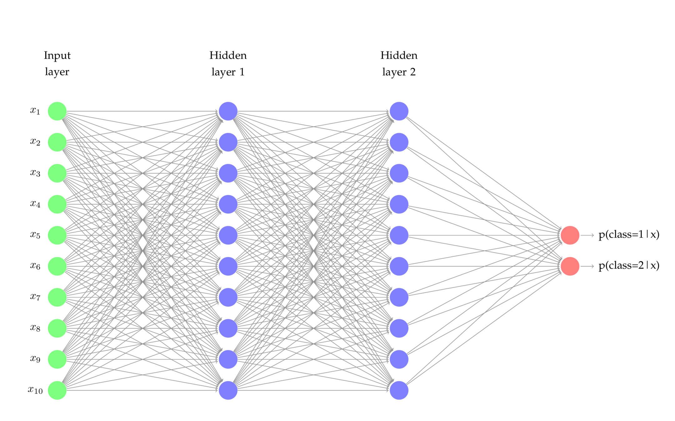
MLP in torch

require "nn"
mlp = nn.Sequential(); 
inputs = 5; outputs = 10;
HUs = {20 , 40}; 
mlp:add(nn.Linear(inputs, HUs[1]))
mlp:add(nn.Tanh())
mlp:add(nn.Linear(HUs[1], HUs[2]))
mlp:add(nn.Tanh())
mlp:add(nn.Linear(HUs[2], outputs))

criterion = nn.MSECriterion()

for i = 1,5000 do
  -- same backprop. routine
end

nn.Sequential {
  [input -> (1) -> (2) -> 
(3) -> (4) -> (5) -> output]
  (1): nn.Linear(10 -> 20)
  (2): nn.Tanh
  (3): nn.Linear(20 -> 40)
  (4): nn.Tanh
  (5): nn.Linear(40 -> 4)
}

Fully connected layer 

• Think of it as a dimension transformation layer/model
• Delineates function approximation
• Used for variant classification tasks

convolutional layer

• A Linear layer requires the input to have a meaning
  • It then extracts linear (or thanks to activation functions, non-linear) relations (of arbitrary dimension) from that data
  • Feature extraction used to be an important part of any machine learning system 
• Convolutional layers do not assume the data to have any meaning

convolutional layer

• Regardless of the dimension, a number of fixed size kernel is convoluted through the input

Input Matrix

• Each Convolution Kernel can be trained to perform a specific task, edge detection etc.

convolutional layer

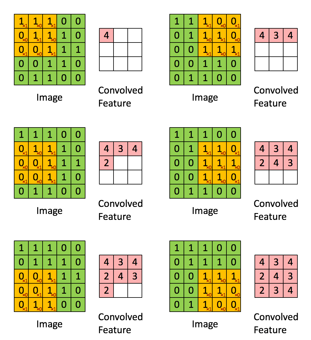
convolutional layer

• Unlike [old-fashioned] feature extraction, where WE decide what features are important to the network, ConvNets decide themselves what is important and what isn't, depending on the task.
• It makes sense: 
  • We memorize (or intuitively know) different features for different tasks
  • We accumulate features that we've seen to make a decision, not all at once.

Other important layers

• A network isn't only made of ConV and Linear layers
  • Activation function
    • ReLU
    • Sigmoid
    • Tanh
  • Downsampling functions 
    • Max-Pooling 
  • Output
    • (Log)SoftMax

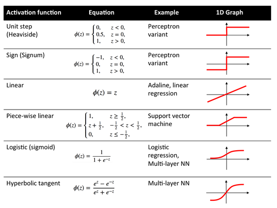
Activation functions

• Introduce Non-linearity to a model with Linear layers
• non-linear means that the output cannot be reproduced from a linear combination of the inputs
• from the generalization point of view, with no non-linear activation function a 3 layer MLP would have performed  tasks just like a single perceptron (~ singe matrix)
• Used after various layers to make the layer's output, which is the input to the next layer capable, of delivering new meanings

Activation functions

Downsampling - max pooling

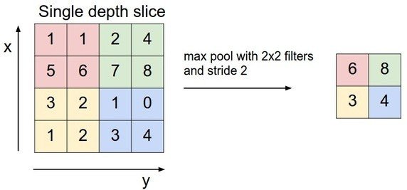
• Avoid over-fitting. The network will not learn solid abstract patterns of the input shape.
• (somehow) force the network to generalize
• Reduce computational cost

output layer - softmax

• A means of replacing SCORE
• By rescaling them so that the elements of the n-dimensional output lie in the range (0, 1) and sum to 1
• Logsoftmax is to take the log() of the softmax output vector, such that elements will not be too small. Each element in the Logsoftmax output can still denote the score of being one class.
• Logsoftmax may be used to prevent underflow.

experiments

ConvNets and more

language and framework

• Lua: a powerful, efficient, lightweight, embeddable scripting language. It supports procedural programming, object-oriented programming, functional programming, data-driven programming, and data description.
  • Lua is distributed in a small package and builds out-of-the-box in all platforms that have a standard C compiler
  • Lua is fast: To claim to be "as fast as Lua" is an aspiration of other scripting language.

language and framework

• Torch: Torch is a scientific computing framework. It is easy to use and efficient, thanks to an easy and fast scripting language, LuaJIT, and an underlying C/CUDA implementation.
  • a powerful N-dimensional array, aka. Tensor
  • Fast and efficient GPU support
  • Embeddable, with ports to iOS, Android and FPGA backends
  • Lots of support from both industry and research groups:
    • Harvard NLP
    • Baidu Research (silicon valley AI Lab.)
    • Facebook AI
    • Twitter AI

machine-generated dataset

• 1177 Farsi fonts
• 32 Character alphabet + 10 numbers
• 40780 images, 1 * 30 * 30 each 
• Cropped, to specific post processing (CNN!)

experiment #1: Vanilla cnn

nn.Sequential {
  [input -> (1) -> (2) -> (3) -> (4) -> (5) -> (6) -> (7) 
-> (8) -> (9) -> (10) -> (11) -> (12) -> (13) -> (14) -> (15) -> (16) -> output]
  (1): nn.SpatialConvolution(1 -> 64, 5x5)
  (2): nn.ReLU
  (3): nn.SpatialConvolution(64 -> 128, 5x5)
  (4): nn.ReLU
  (5): nn.SpatialConvolution(128 -> 128, 5x5)
  (6): nn.ReLU
  (7): nn.SpatialMaxPooling(2x2, 2,2)
  (8): nn.View(10368)
  (9): nn.Linear(10368 -> 512)
  (10): nn.ReLU
  (11): nn.Linear(512 -> 256)
  (12): nn.ReLU
  (13): nn.Linear(256 -> 128)
  (14): nn.ReLU
  (15): nn.Linear(128 -> 40)
  (16): nn.LogSoftMax
}

experiment #1: Vanilla cnn

• Validation ratio: 20%
• Validation accuracy: ~89%
• Example Kernel: Terminal

1.8489112831681e-06	ا	
8.5918503451228e-07	ب	
9.9835042715169e-06	پ	
2.911008198596e-06	ت	
6.9377831794647e-07	ث	
4.2834721628495e-05	ج	
0.99981760314176	چ

improvements:

• Batch normalization 
• Dropout 
• Padded Convolution layer
• Stronger Activation function
• More layers and depth

EXPERIMENT #2: OPTIMIZED CNN 

nn.Serial @ nn.Sequential {
  [input -> (1) -> (2) -> (3) -> (4) -> (5) -> (6) -> (7) -> (8) -> (9) -> (10) -> (11) -> (12) -> (13) -> (14) -> (15) -> (16) -> (17) -> (18) -> (19) -> (20) -> (21) -> (22) -> (23) -> (24) -> output]
  (1): nn.Convert
  (2): nn.SpatialDropout(0.200000)
  (3): nn.SpatialConvolution(1 -> 64, 5x5, 1,1, 2,2)
  (4): nn.SpatialBatchNormalization
  (5): nn.Tanh
  (6): nn.SpatialMaxPooling(2x2, 2,2)
  (7): nn.SpatialDropout(0.500000)
  (8): nn.SpatialConvolution(64 -> 128, 5x5, 1,1, 2,2)
  (9): nn.SpatialBatchNormalization
  (10): nn.Tanh
  (11): nn.SpatialMaxPooling(2x2, 2,2)
  (12): nn.Collapse
  (13): nn.Dropout(0.500000)
  (14): nn.Linear(6272 -> 512)
  (15): nn.BatchNormalization
  (16): nn.Tanh
  (17): nn.Linear(512 -> 256)
  (18): nn.BatchNormalization
  (19): nn.Tanh
  (20): nn.Linear(256 -> 128)
  (21): nn.BatchNormalization
  (22): nn.Tanh
  (23): nn.Linear(128 -> 40)
  (24): nn.LogSoftMax
}

tanh activation function

• Older, (in some cases)stronger than ReLU
• unified mean and standard deviation
• Tanh seems maybe slower than ReLU for many of the given examples, but produces more natural looking fits for the data using only linear inputs, as you describe
• http://playground.tensorflow.org/

Batch normalization

• your first layer parameters change and so the distribution of the input to your second layer changes unified mean and standard deviation, "internal covariate shift"
• To remedy internal covariate shift, the solution proposed is to normalize each batch by both mean and variance
• Note that this is in no way similar to helping the model memorize.
• It's actually a method to generalize.

dropout

• Dropout is a technique where randomly selected neurons are ignored during training
• This means that their contribution to the activation of downstream neurons is temporally removed on the forward pass and any weight updates are not applied to the neuron on the backward pass

• Validation ratio: 20%
• Validation accuracy: ~96%

improved results

References

• Batch Normalization: https://arxiv.org/pdf/1502.03167v3.pdf
• Dropout: https://www.cs.toronto.edu/~hinton/absps/JMLRdropout.pdf
• TanH, ReLU and Backprop: http://yann.lecun.com/exdb/publis/pdf/lecun-98b.pdf 

cnn in the wild

synthetic dataset

• Machine generated text
• Handwritten recognition 

experiments

dataset

• Text modification: 
  • Invert pixel value
  • Stroke vs. Fill
  • Normalize ~ gray 
• All changes take place according to a probability
• Results in around 90k images

The aim is to train the system on computer fonts and test it on handwritten text. In oder words, claim that such dataset is enough to generalize the model to a greater scope

0.00015779999353047	د	
3.521212034443e-07	ذ	
0.0014876711478155	ر	
1.5775675775864e-05	ز	
2.7149472579572e-05	ژ	
0.97940942162196	س	
0.0006677035107906	ش	
0.0024584838050561	ص	
1.9488518805953e-05	ض	
3.917732601588e-05	ط

0.00074010179250526	ت	
0.021139973753066	ث	
0.55511346194901	ج	
0.00092499923480925	چ	
0.0015544320115577	ح	
0.017658120147062	خ	
0.020682373658584	د	
0.00085717213848045	ذ	

recurrent layers

• The idea behind CNN was to capture SPATIAL features
• RNN expands this further into TEMPORAL features
• Used for Sequence to Sequence, Vector to Sequence etc. tasks. In other words, whenever the input data has temporal dependency/meaning, it can be fed into the network as a time-indexed sequence.
• Think of language model as an example.

recurrent layers

feedforward network

recurrent layers

recurrent neuron: simple example

recurrent layers

• A Recurrent network processes data through time
• It keeps a memory of what it has already seen and outputs w.r.t to its history and internal weights
• Back propagation Through Time: Vanishing Gradient
  • Due to numerous multiplication, gradients tend to be very small. Solution:
    • LSTM Layers
    • Gated Recurrent Units
  • From our point of view, all of them can be deemed as recurrent layers with same input output.

references

• GRU and LSTM: https://arxiv.org/pdf/1412.3555v1.pdf
• LSTM step by step: http://colah.github.io/posts/2015-08-Understanding-LSTMs/

encoder - decoder archtecture

• The encoder-decoder models in context of recurrent neural networks (RNNs) are sequence to sequence mapping models
• The encoder network is that part of the network that takes the input sequence and maps it to an encoded representation of the sequence. The decoder then uses this encoded data to generate a sequence of output.
• Renowned for impressive performance in translation
• The encoder replaces yet another feature extraction step, namely Word/Sentence Embedding.

encoder - decoder archtecture

encoder - decoder archtecture

references: 

• https://www.tensorflow.org/tutorials/seq2seq/
• https://arxiv.org/pdf/1406.1078.pdf

attention based decoding

so far ...

• We did a great job of replacing spatial feature engineering with learnable convolutional kernels
• We replaced temporal relations with a learnable encoded vector produced by the encoder
• Although the decoder architecture that we saw earlier is learnable, 
• It's unfair to expect it to decode all of the information from a single vector
• If only we could apply more learnability and sophistication to the decoding process...

attention based decoding

• With an attention mechanism we no longer try encode the full source sentence into a fixed-length vector. Rather, we allow the decoder to “attend” to different parts of the source sentence at each step of the output generation

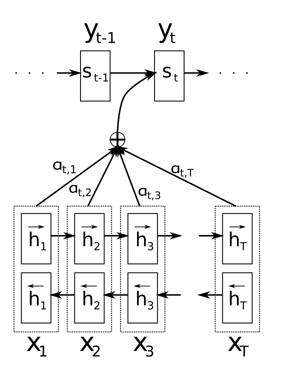
references: 

• http://stanford.edu/~lmthang/data/papers/emnlp15_attn.pdf
• https://arxiv.org/pdf/1406.6247v1.pdf
• https://arxiv.org/abs/1502.03044​

experiments

Sequence to Sequence, end-to-end text recognition

dataset

• ~100K valid sentences
• ~ 300K words extracted 
• ~40 fonts
• 4 synthetic modified extensions with probability 
• ~ 2.5M images generated. 
• 1M used in this experiment. Expensive computation
• 80K validation set
• 91% acc. after 10 epochs

step by step through the model

results

باصعودارسنال

شادی

رونمایی

خرداد

درصد

کیاب

بینایی

ماشین

مباز

کبن