From random forests to regulatory rules: interpreting supervised learners to guide biological discovery
Karl Kumbier
UC Berkeley Statistics
Advisor: Prof. Bin Yu
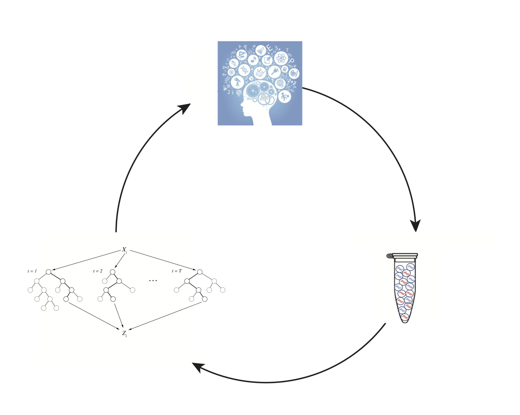
Generating insights in biology through domain-inspired statistical machine learning
Domain knowledge
Modeling/
analysis
Experimental design/data collection
In collaboration with: Susan Celniker (LBNL), James B. Brown (LBNL)
The PCS framework: evaluating human judgement calls in data science
- Predictability: Does my model reflect external reality?
- Computability: Can I tractably build/train my model?
- Stability: Are my results consistent with respect to "reasonable" perturbations of the data/model?
Outline
-
From genomic to statistical interactions
-
Market baskets and genomics
-
Iterative Random Forests
-
Case studies in Drosophila development
From genomic to statistical interactions
Embryonic development in Drosophila
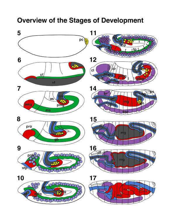


0-1:20 hours
1:20-3:00 hours
3:00-3:40 hours
3:40-5:20 hours
5:20-9:00 hours
9:20-16:00 hours
image: Volker Hartenstein
images: BDGP
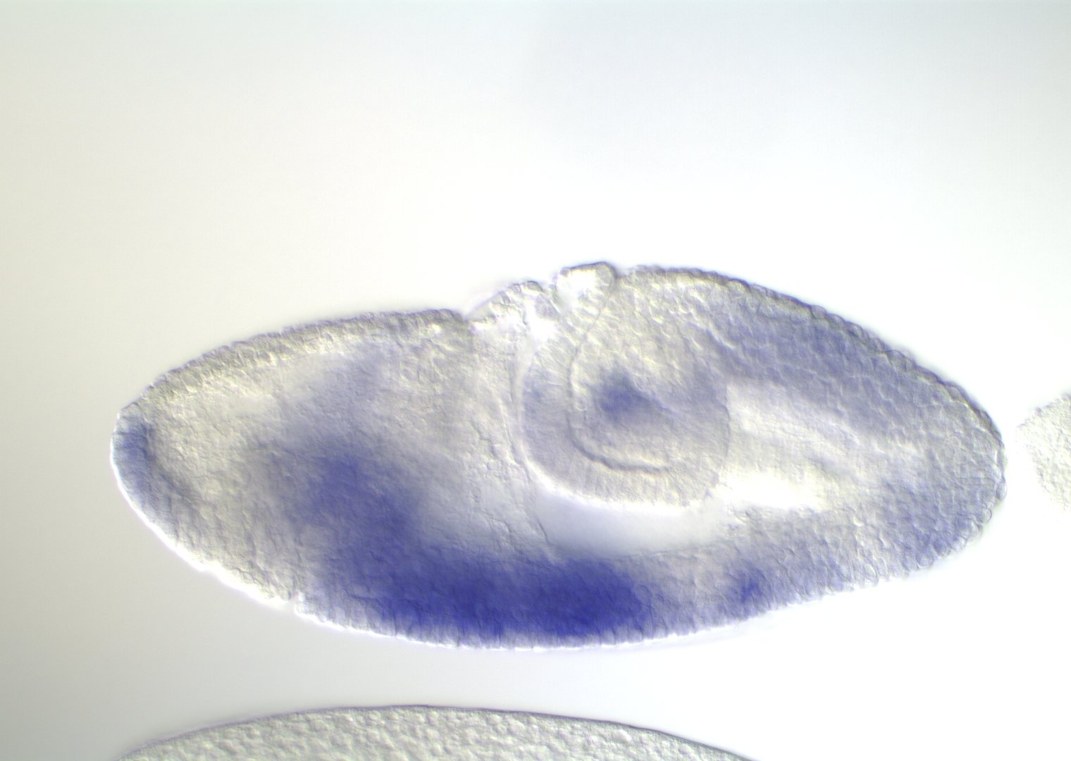
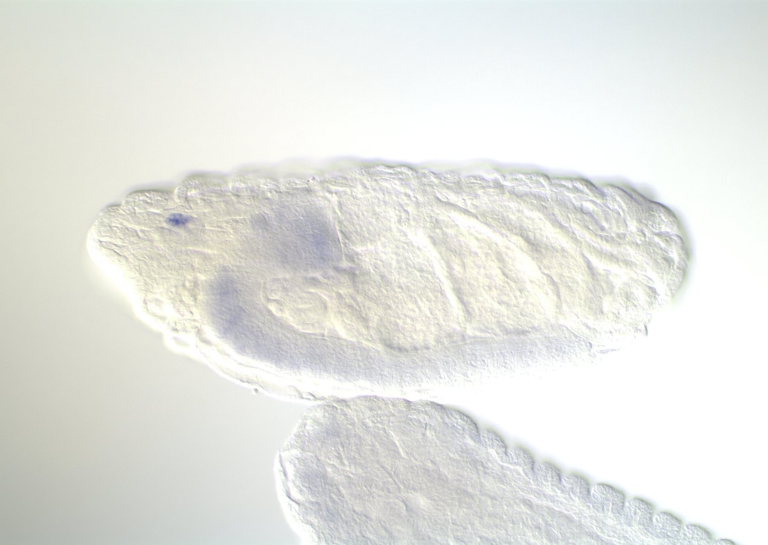
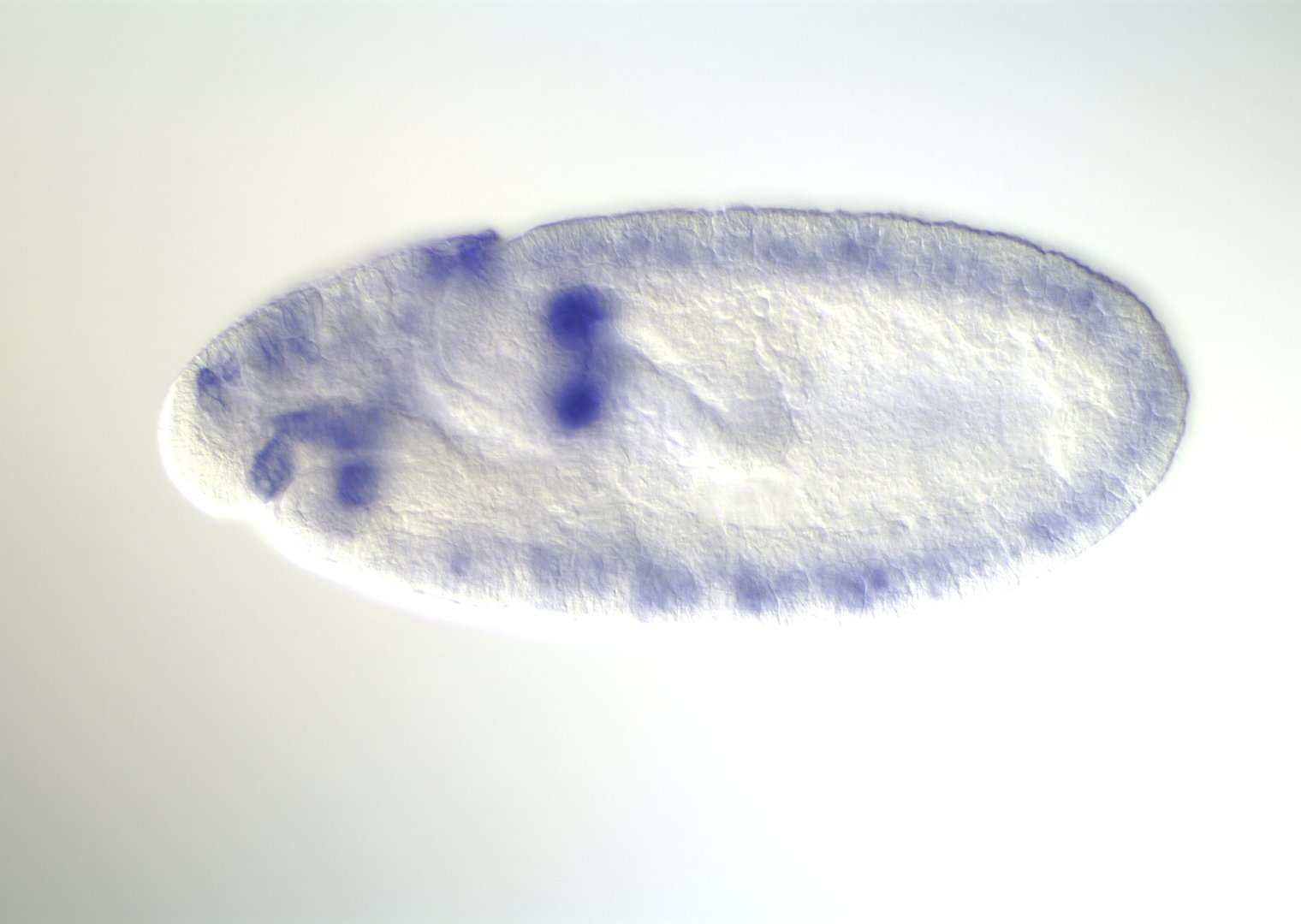
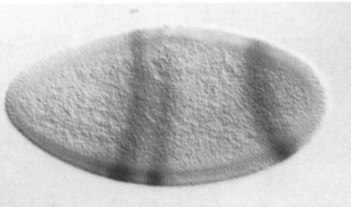
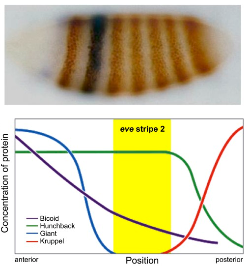
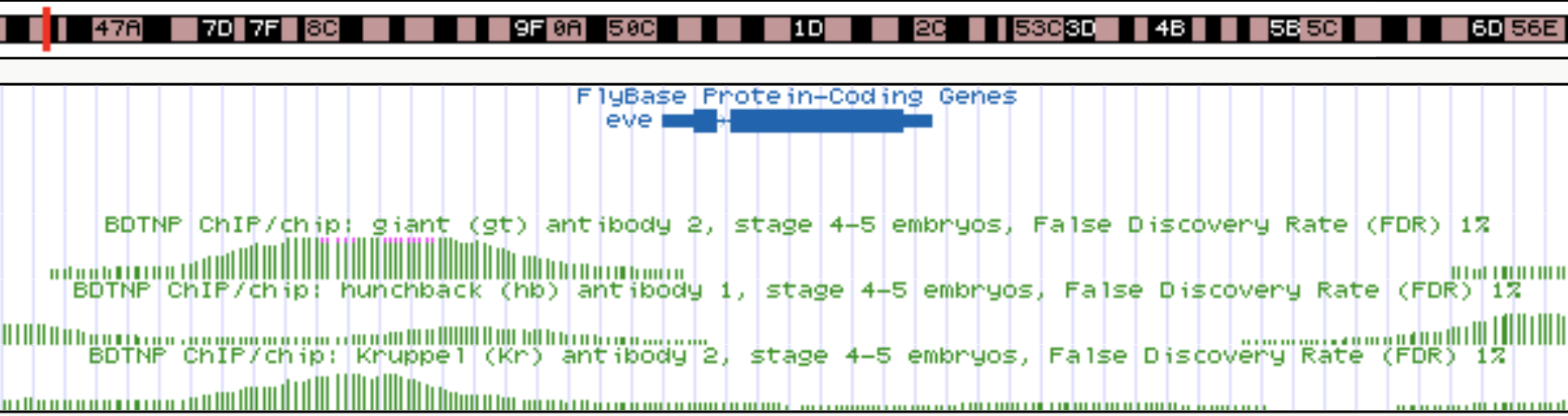
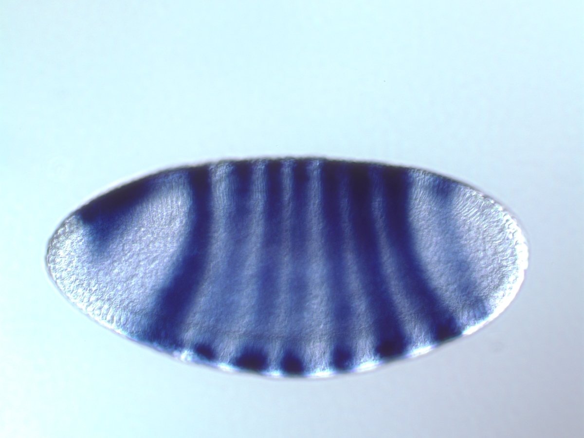
Kr expression
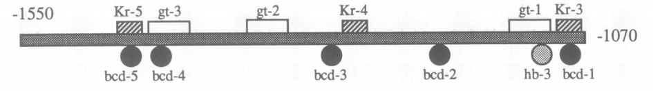
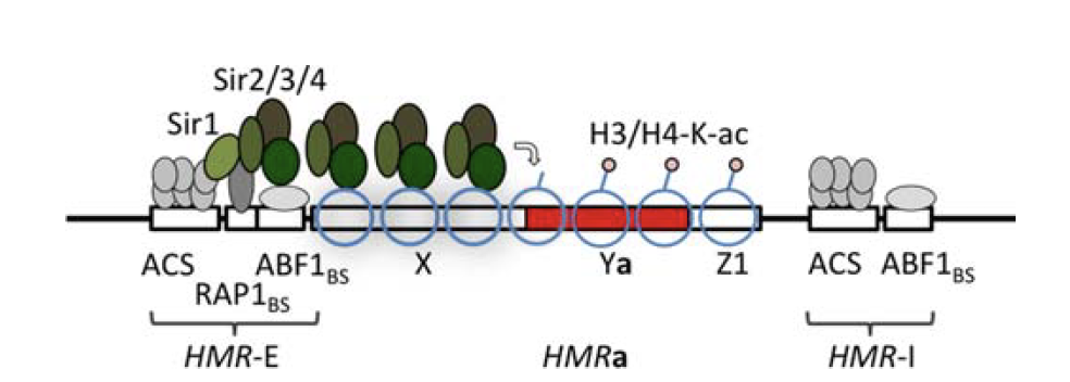
Enhancers regulate spatio-temporal programs of gene expression
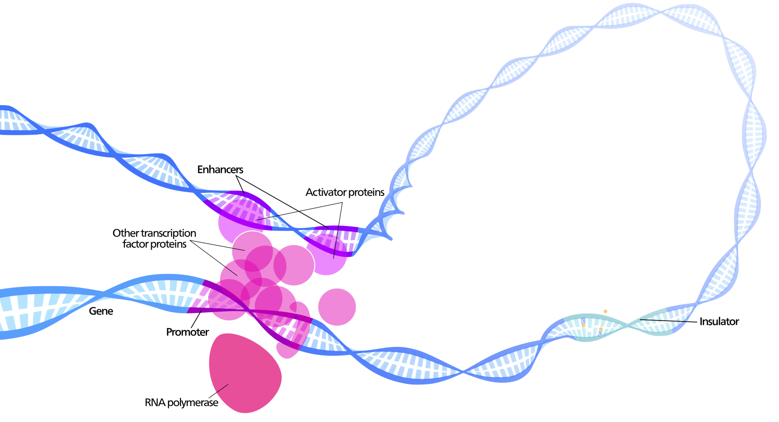
Enhancers: segments of the genome that coordinate transcription factor (TF) activity to regulate gene expression.
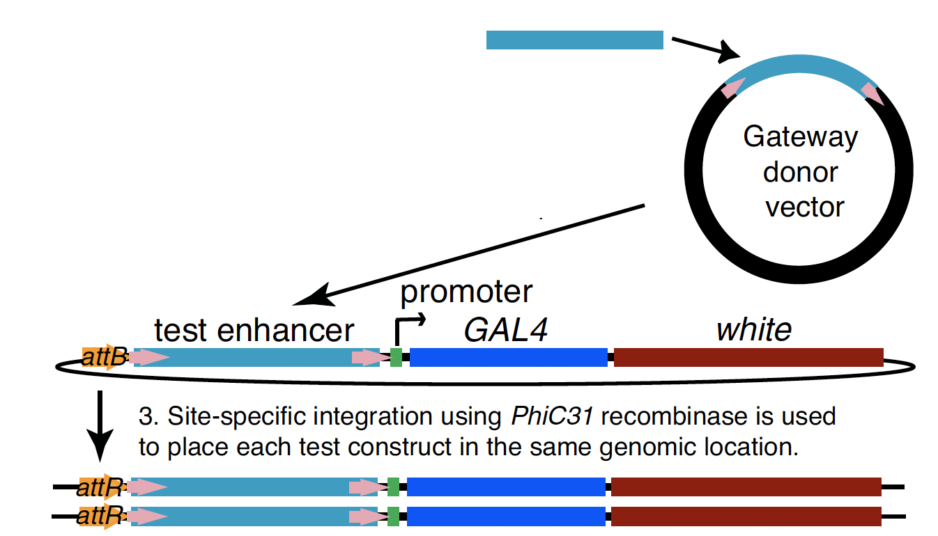
Experimental evaluation of enhancer elements in Drosophila
Pfeiffer et al. (2008)
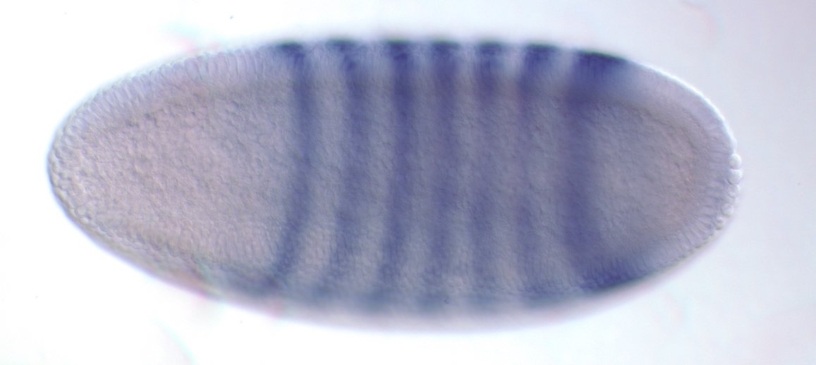
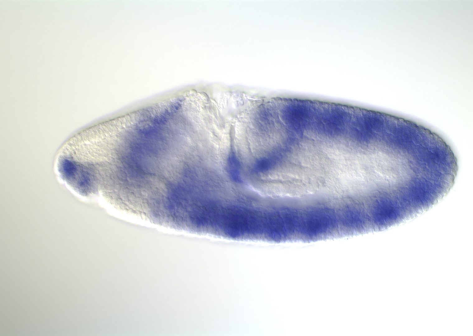
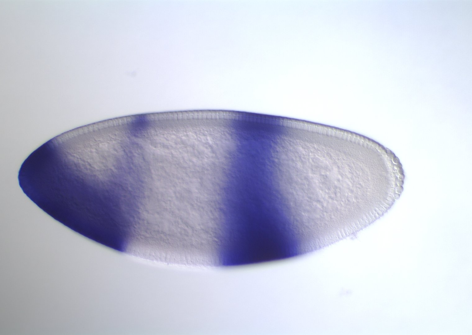
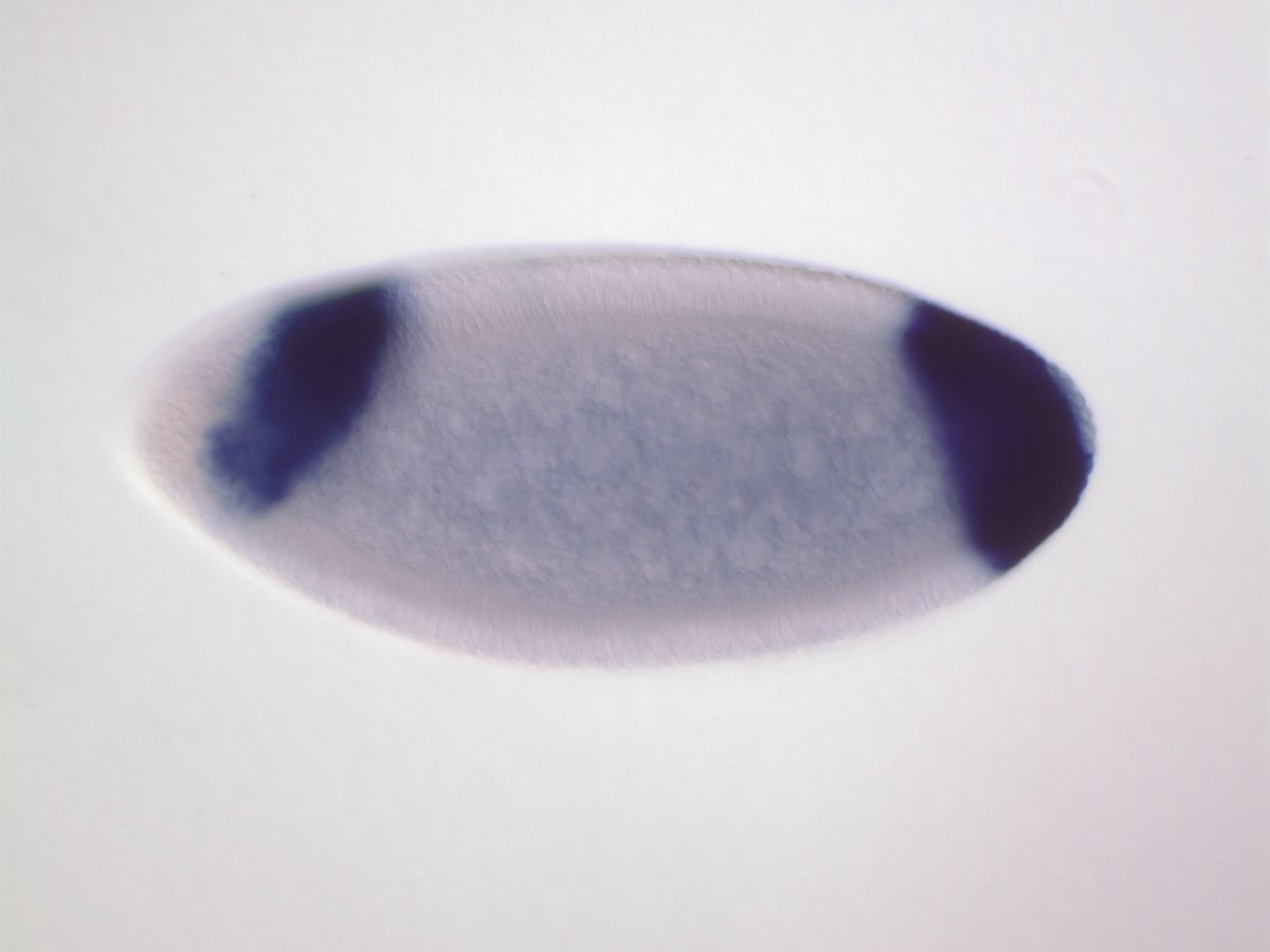
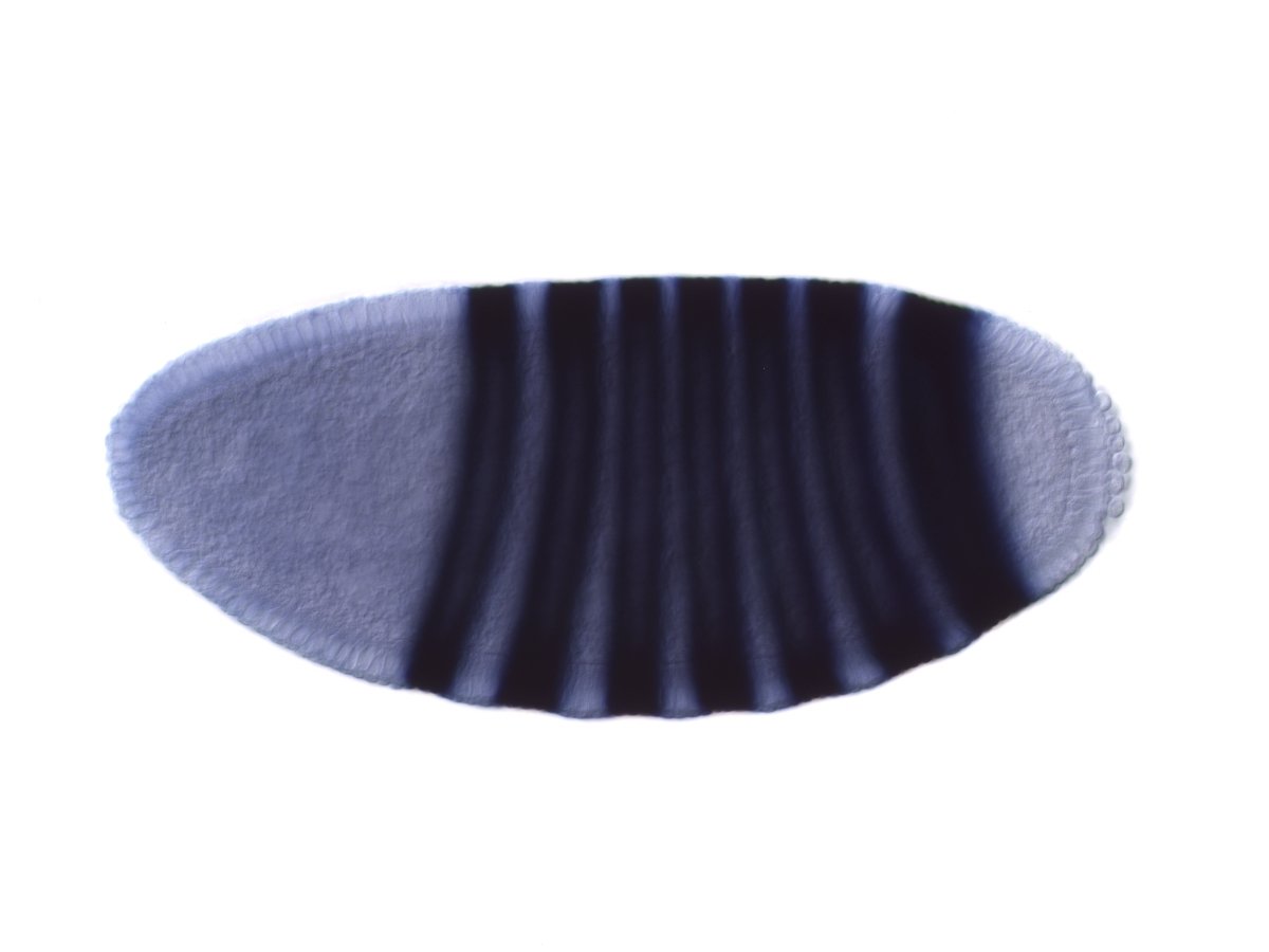
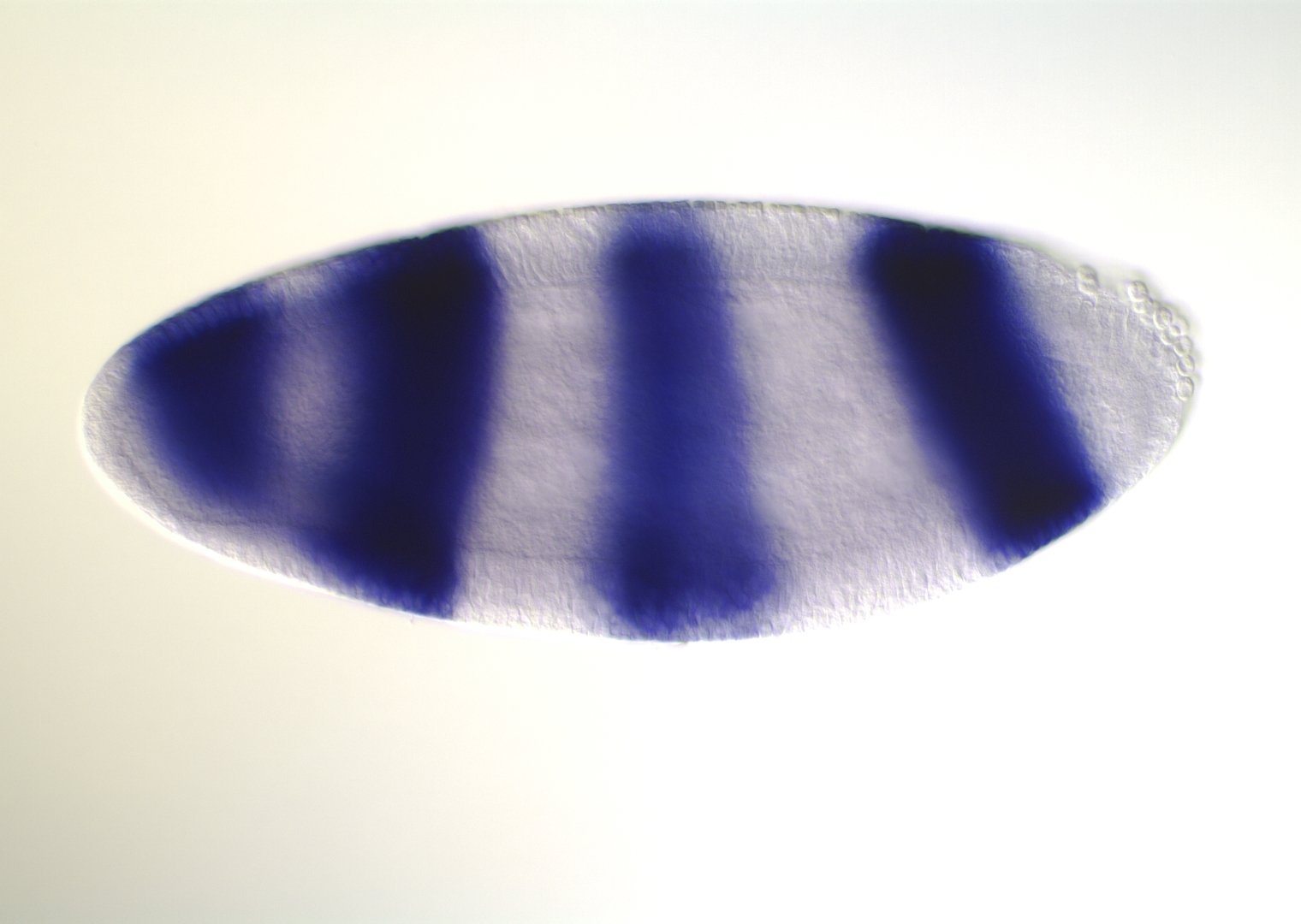
even-skipped
expression
wt
transgenic
Experimental evaluation of enhancer elements in Drosophila
Hiromi et al. (1985), Harding et al. (1989), Goto et al. (1989), Pfeiffer et al. (2008)
even-skipped expression
wt
transgenic
High-order interactions at enhancer elements drive embryonic development
Goto et al. (1989), Harding et al. (1989), Small et al. (1992), Isley et al. (2013), Levine et al. (2013)
Identifying regulatory interactions from high-throughput genomic data
Experimentally validated enhancer elements.
Whole-embryo ChIP-chip/ChIP-seq measurements of transcription factor (TF) DNA binding

From genomic to statistical interactions
activators
repressors
Segment of the genome
DNA binding for p transcription factors (TFs)
Order-s interaction: s = #activators + #repressors

Thresholding rules define expression domains
Chopra and Levine (2009)
Dl +
Dl -
Wolpert (1968), Jaeger and Reinitz (2006), Chopra and Levine (2009), Zizen et al. (2009), Knowles and Biggin (2013), Levine (2013), Staller al. (2015), ...
Jaeger and Reinitz (2009)
From genomic to statistical interactions
(1) How precisely does an interaction predict class-1 observations?
(2) How prevalent is an interaction among class-1 observations?
Interactions:
Responses:
?
RuleFit: rule-based interaction discovery (Friedman and Popescu, 2008)
- Identify a collection of marginally important features
- Search for predictive order-2 rules among marginally important features
Computational costs grow as
Misses interactions with weak marginal effects
image: Lee and Haber (2014)
Market baskets and genomics
Interactions in market baskets


What combinations of items do customers purchase together?
Interactions in market baskets
What combinations of items do customers purchase together?
What combinations of items do different types of customers purchase together?


Interactions in market baskets
Feature-index sets
Random intersection trees (RIT)
Shah and Meinshausen (2014)
Leverage sparsity in market baskets to search for frequently co-occurring items in a computationally efficient manner
- Randomly sample feature index sets from class-C observations:
- Intersect sampled feature index sets in a tree like fashion up to depth D
- Return all feature combinations that "survive" intersection procedure up to depth D
Random intersection trees (RIT)
Shah and Meinshausen (2014)
Randomly sampled
class-C observation
"survived" interaction
Random intersection trees (RIT)
Shah and Meinshausen (2014)
Random intersection trees (RIT)
Shah and Meinshausen (2014)
Genomic response
Genomic features
Translating the market basket problem into genomics

Genomic response
Genomic features
Translating the market basket problem into genomics
Challenges:
- Genomic features are typically measured in concentrations/counts
- Binding does not imply regulation (Li et al. 2008)
iterative Random Forests (iRF)
&
signed iterative Random Forests (s-iRF)
Joint work with Sumanta Basu, James B. Brown, Susan Celniker, and Bin Yu
iterative Random Forest to identify high-order interactions in genomic data
- Iteratively re-weighted Random Forests stabilize decision path
- Generalized random intersection trees search for high-order interactions
- Stability bagging evaluates interactions
iterative Random Forests (iRF) build on PCS to identify genomic interactions in developing Drosophila embryos
Open source R implementation: https://cran.r-project.org/web/packages/iRF/
Iteratively re-weighted random forests
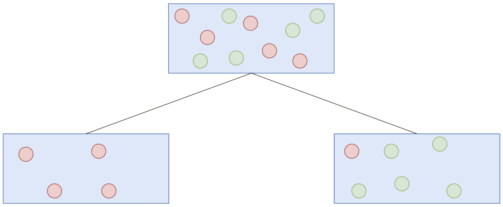
Classification and regression trees (CART)
Breiman et al. (1984)
For current node:
- Select splitting feature and threshold
- Partition data
- Repeat until stopping criteria
Classification and regression trees (CART)
Breiman et al. (1984)
For current node:
- Select splitting feature and threshold
- Partition data
- Repeat until stopping criteria
The CART criterion: Gini impurity
Proportion positive responses
Number of observations
Gini impurity:
Decrease in Gini impurity:
Mean decrease in impurity:
On average, how much does splitting on a variable decrease the Gini impurity?
Random Forests
Breiman (2001)
Random forests modify CART to improve predictive accuracy:
- CART trees are trained on bootstrap samples of the data
- CART criterion evaluated on subset of features sampled uniformly at random
Feature-weighted Random Forests
Amaratunga et al. (2008)
Random forests:
At each node of the decision tree, uniformly sample a subset of features
Feature-weighted random forests:
At each node of the decision tree, sample a subset of features with probability proportional to
Feature weights
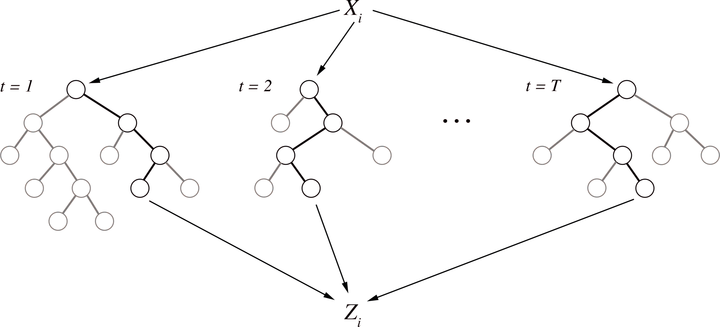
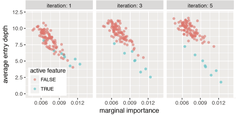
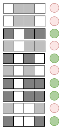
Iterative re-weighting stabilizes random forest decision paths
Gini importance
Iteration 1
Iteration K
Feature weights
Iterative re-weighting helps recover high-order interactions
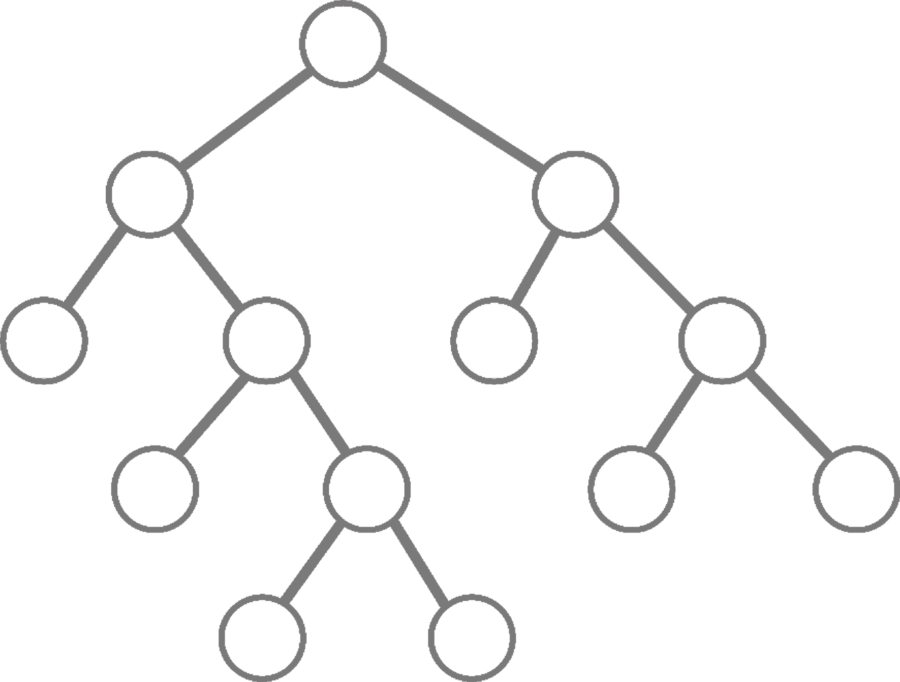
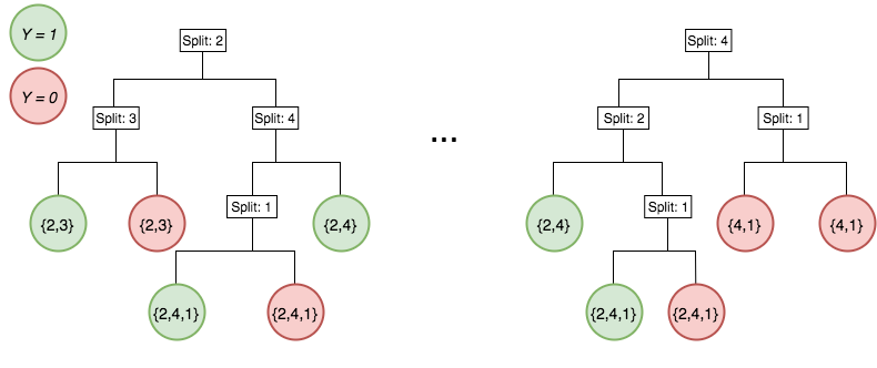
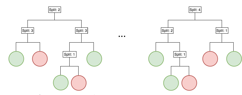
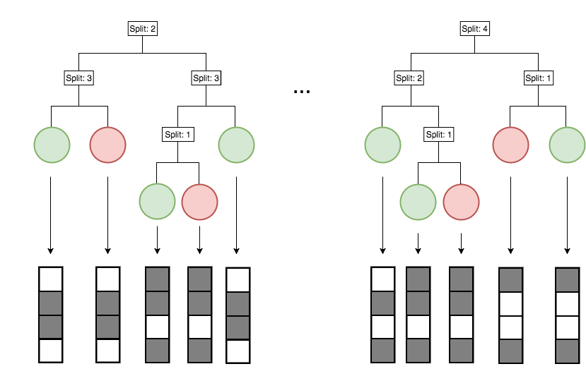
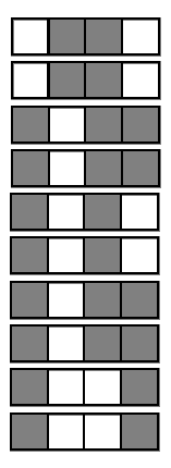
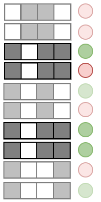
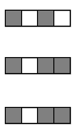
Generalized random intersection trees
Encoding decision paths to extract active features
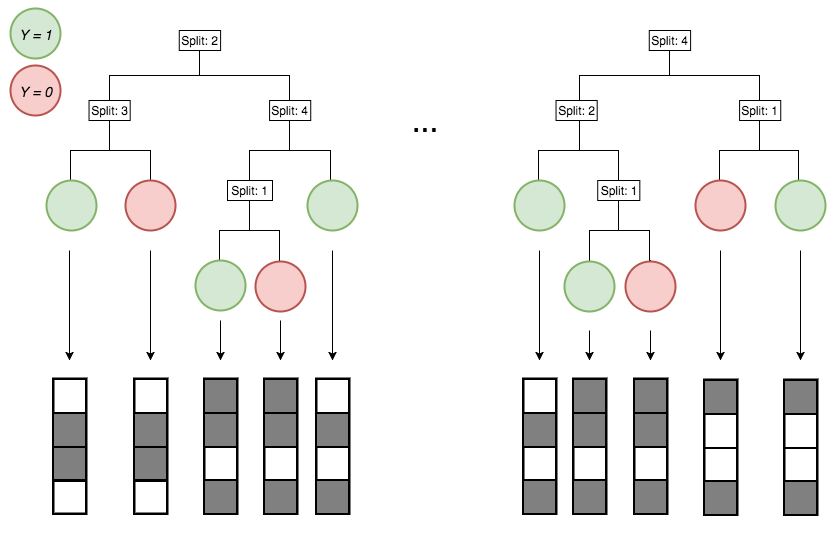
Active
Inactive
Continuous measurements
Binary features

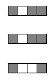
Encoding decision paths to extract enriched and depleted features
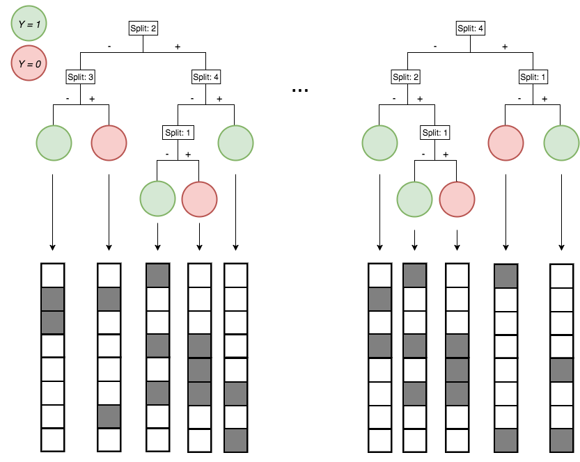
Enriched
Depleted
Generalized random intersection trees search for high-order interactions
1. Iteratively re-weighted random forests
3. RIT on random forest decision paths
2. Decision path feature transformation
.
.
.
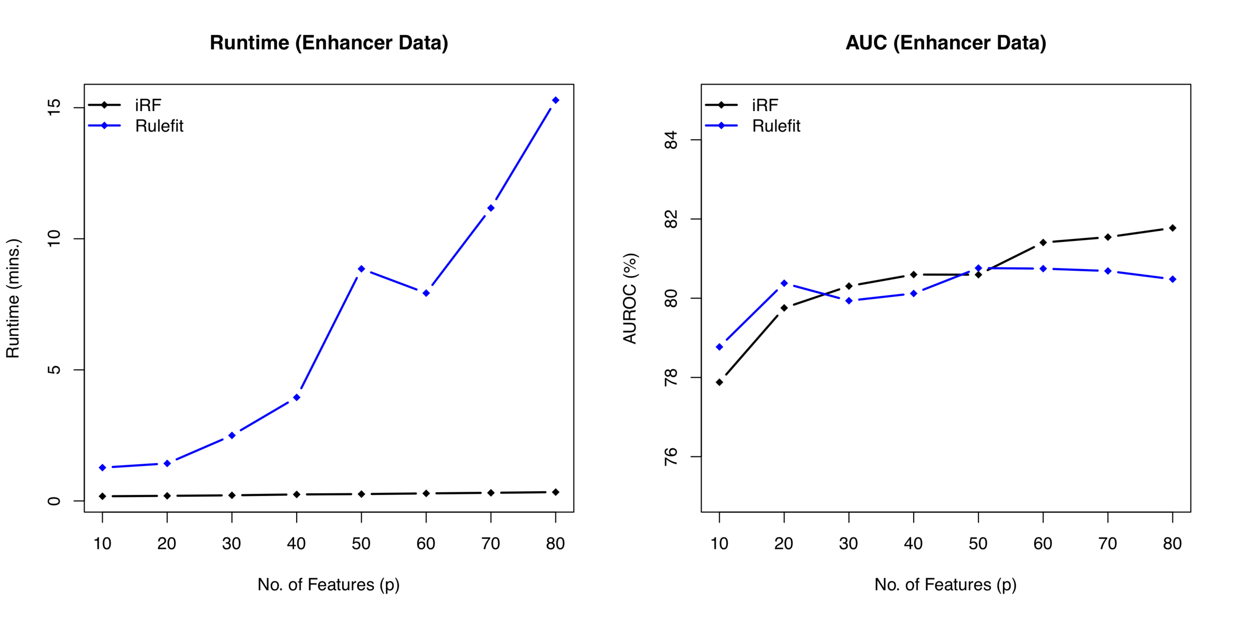
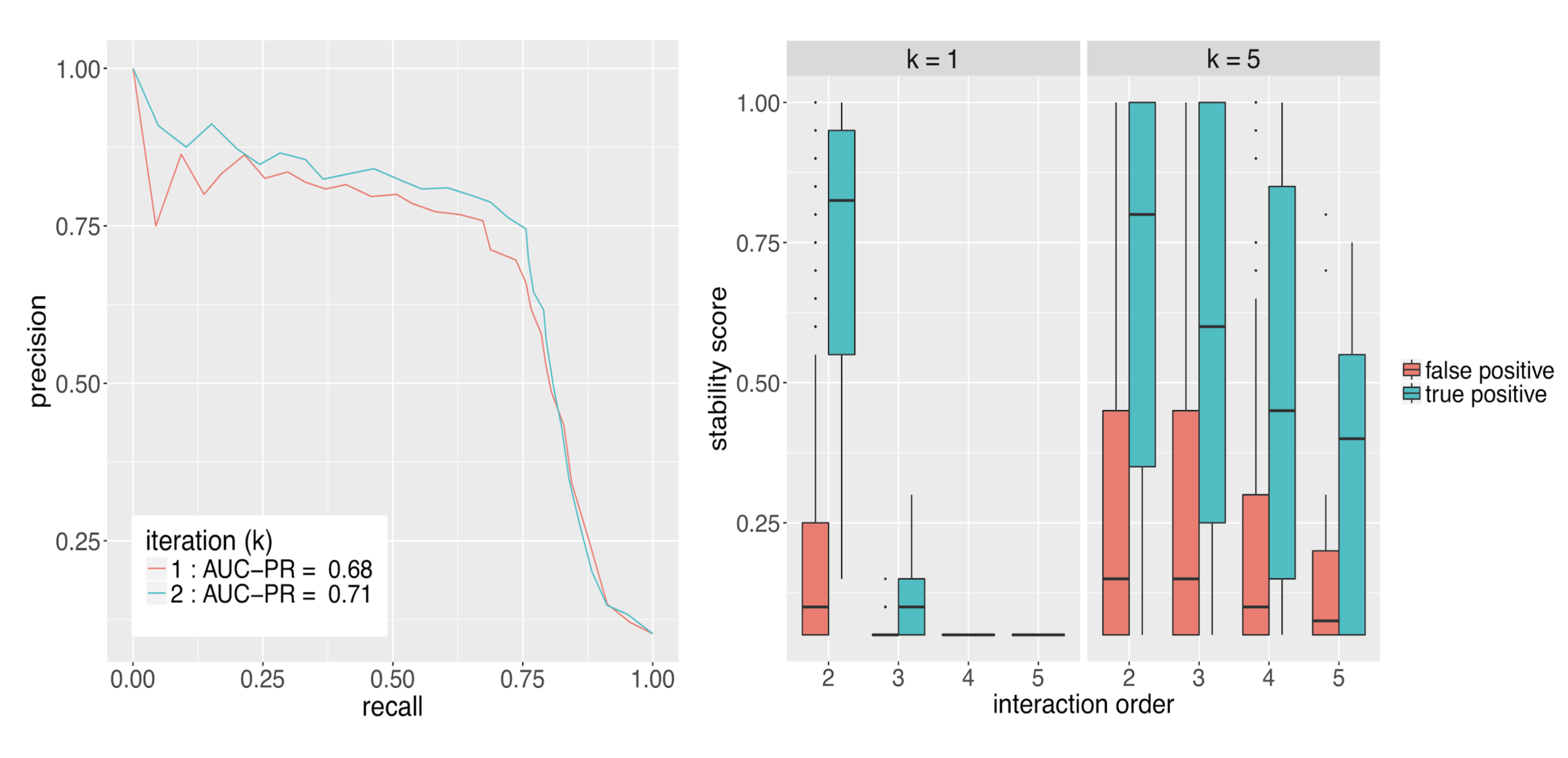
Runtime comparison between iRF and RuleFit
Evaluating interactions
Summary of importance measures for high-order interactions
Importance measures:
- Prevalence : how frequently is an interaction observed among positive responses?
- Precision : how accurately does an interaction predict positive responses?
Null importance measures:
- Class enrichment: is an interaction more prevalent among a particular class?
- Interaction strength: is feature selection dependent on the joint distribution of features?
- Minimal representation: how much do additional features improve prediction accuracy?
Prevalence measures the stability of an interaction across an RF
Prevalence:
Examples:
Precision measures the predictive accuracy of an interaction across an RF
Precision:
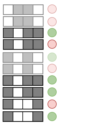
Examples:
Bagging evaluates stability of interactions across entire iRF workflow relative to resampling
1. Iteratively re-weighted RF stabilize decision paths
2. gRIT searches for high-order interactions along decision paths
3. Importance metrics evaluate interactions in fitted RF
Outer layer bootstrap samples
Case studies in Drosophila
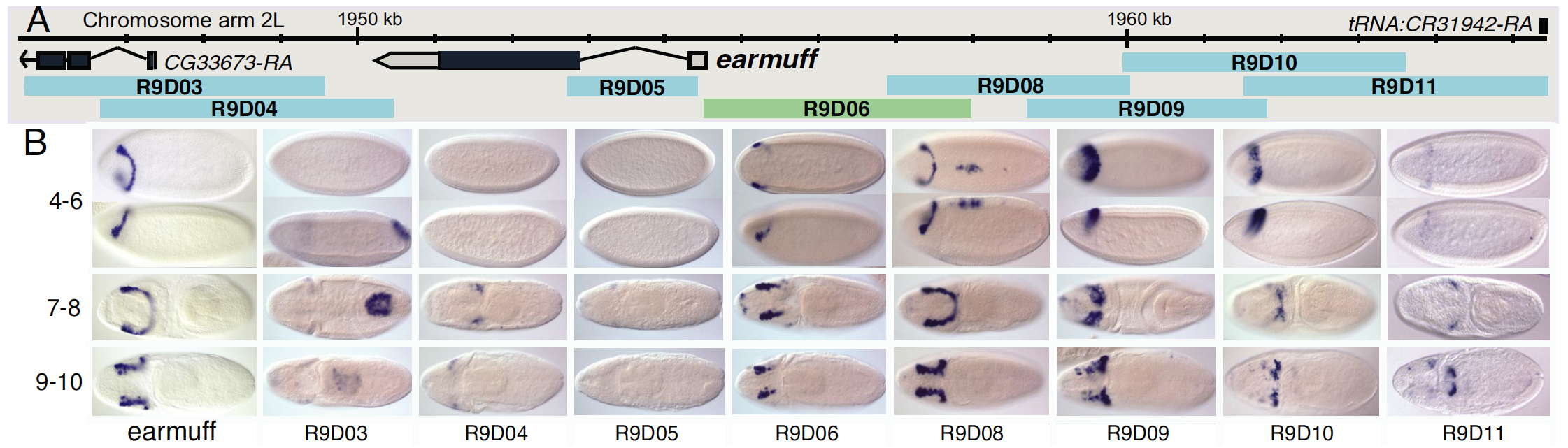
Predicting enhancer activity in early stage Drosophila embryos
Enhancers: Pfeiffer et al. 2008, Fisher et al. 2012, Kvon et al. 2014
ChIP: MacArthur et al. 2009, Li et al. 2008
- 7809 loci representing ~14% of the non-coding genome
- : 24 TF ChIP assays, stage 4-6 blastoderm embryos
- : enhancer activity (0: inactive, 1: active)
Predicting enhancer activity in early stage Drosophila embryos
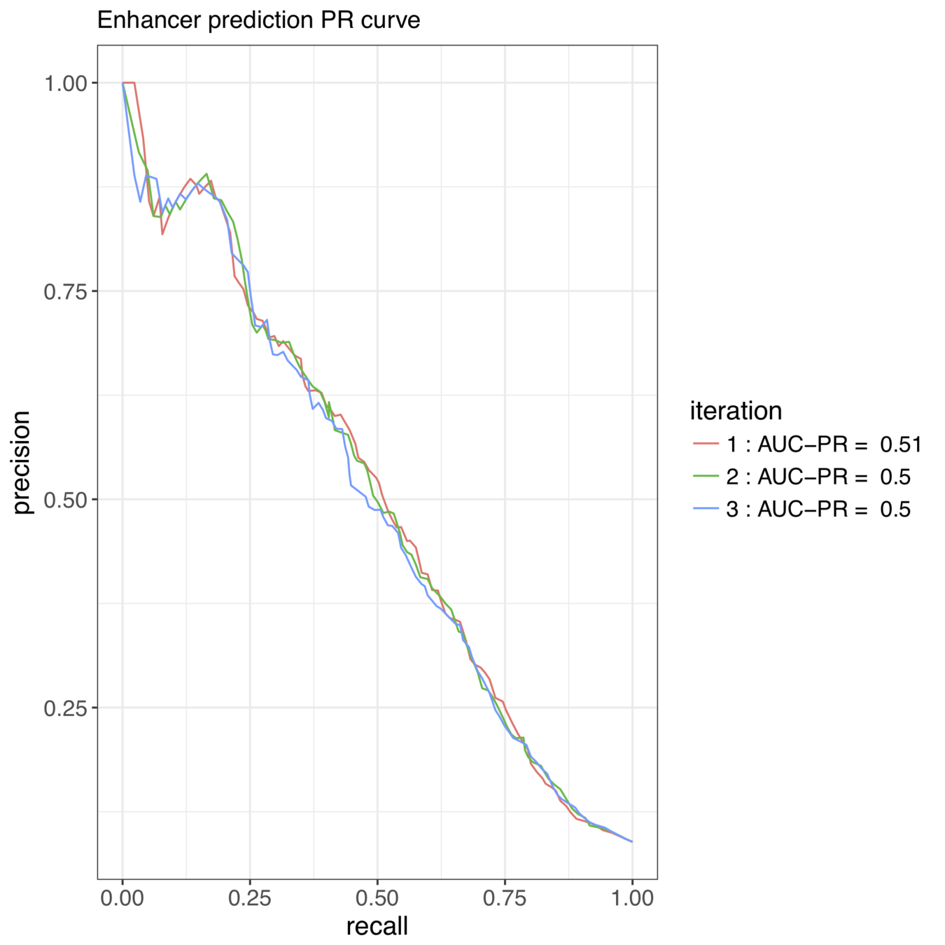
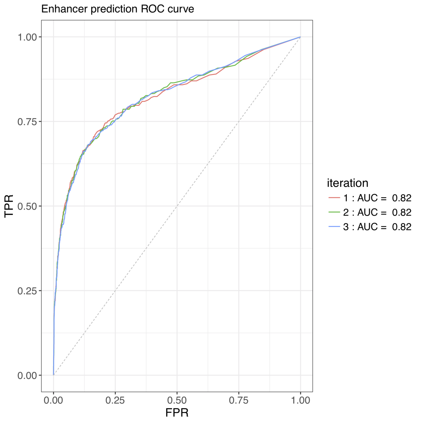
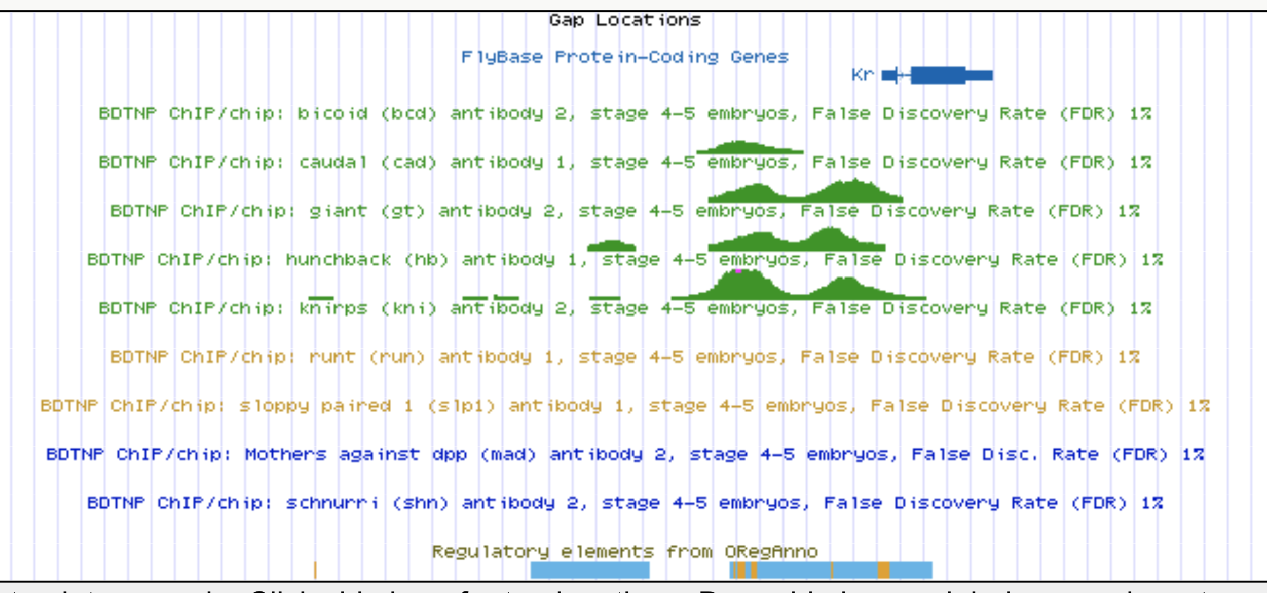
iterative Random Forests recover well-known pairwise interactions
Accurately predicted enhancer elements correspond to A-P expression patterns
active enhancer
Rule predicted probability

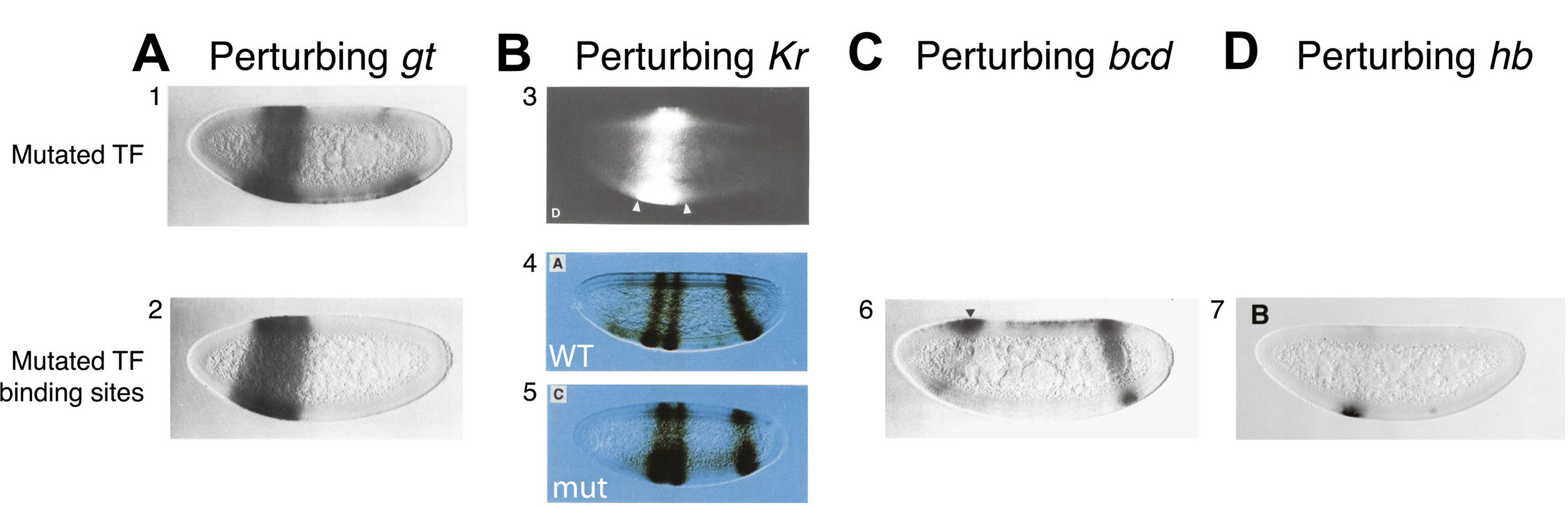
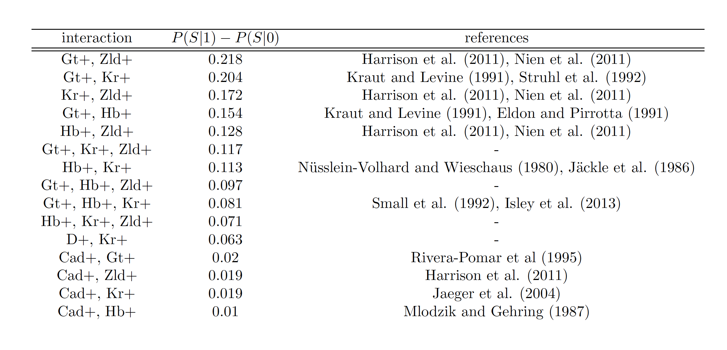
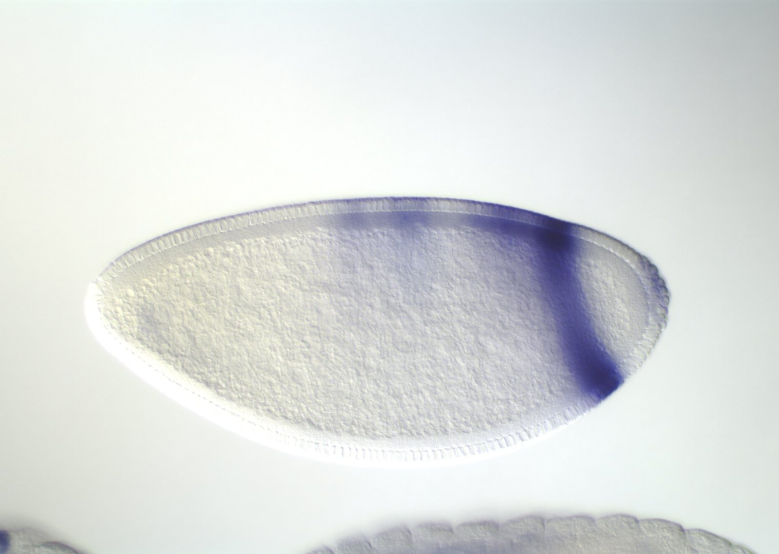
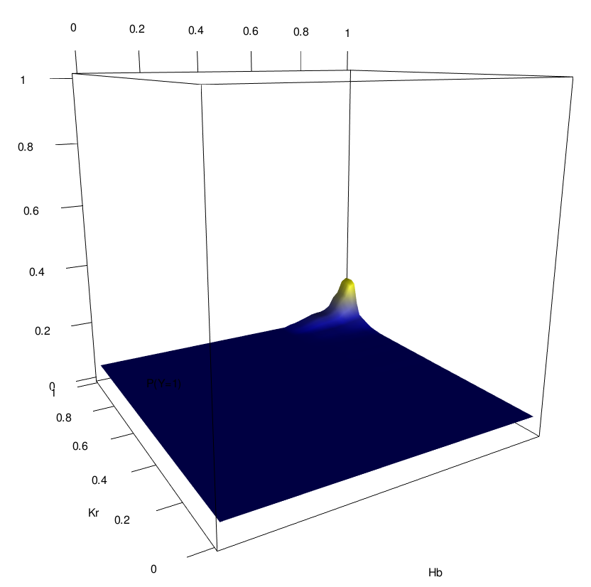
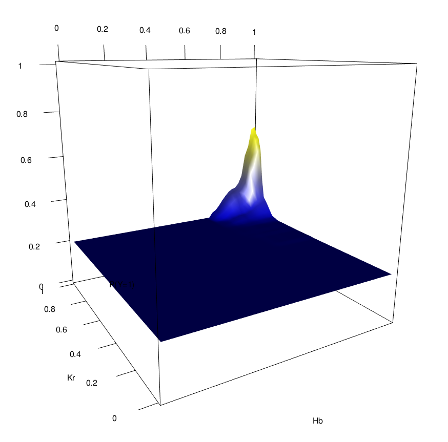
s-iRF identifies known target of order-3 gap gene interaction
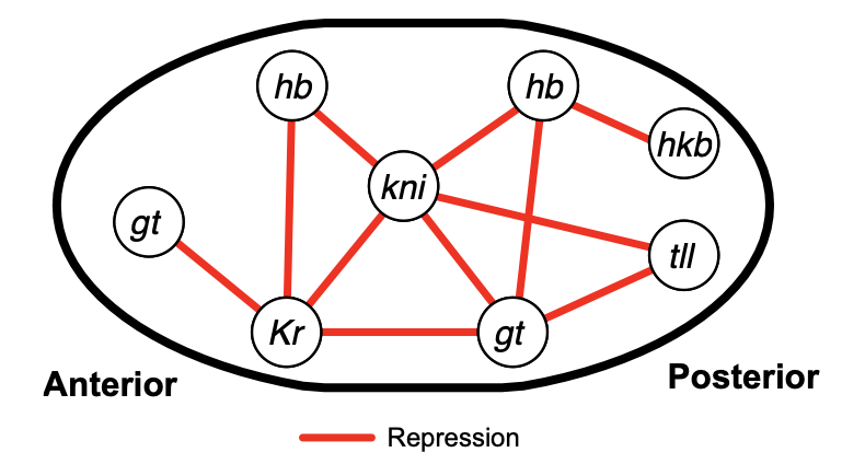
Known target of order-3 interaction among Gt, Kr, and Hb


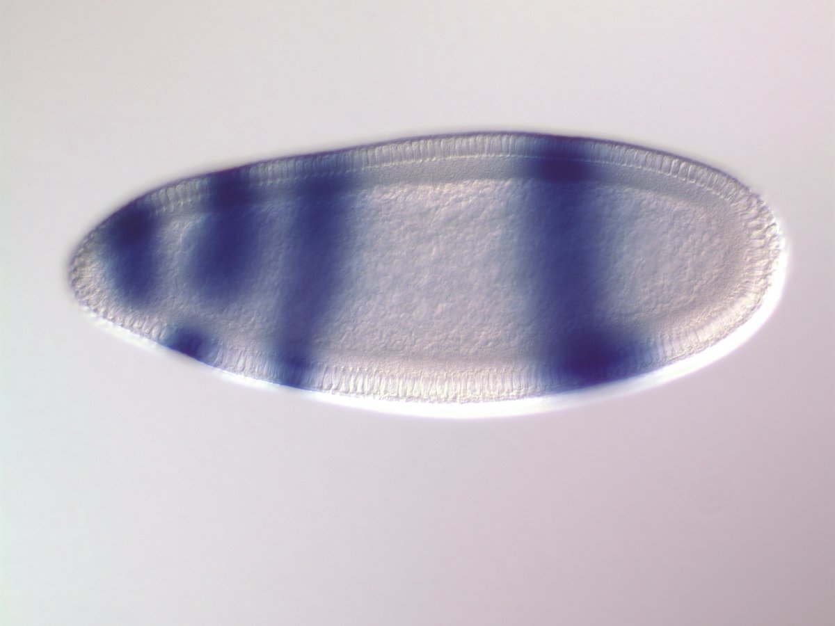
Gt
Kr
Hb
eve
Gt, Kr, Hb binding
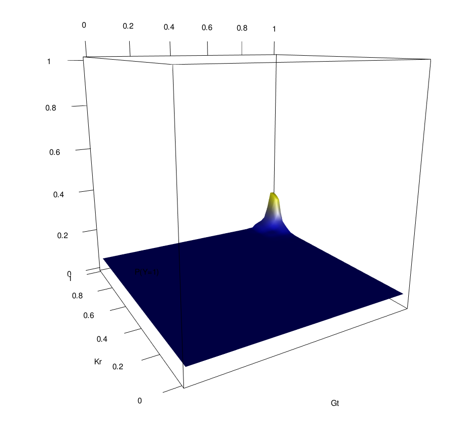
s-iRF suggests novel targets for order-3 gap gene interaction
Gt, Kr, Hb
binding
Known gap gene target
Kni

Gt
Kr
Hb
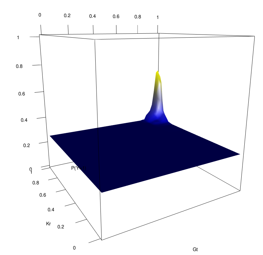
s-iRF suggests novel targets for order-3 gap gene interaction
Gt, Kr, Hb
binding
Known gap gene target
Gt
Kr
Hb


Cad early
Cad late
Novel order-3 interactions exhibit AND-like behavior (Hb, Kr, Zld)
Zld low
Zld high
Hb
Kr
Kr
Hb
Novel order-3 interactions exhibit AND-like behavior (Gt, Kr, Zld)
Zld low
Zld high
Gt
Kr
Kr
Gt
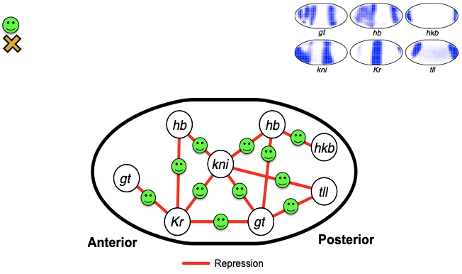
Identifying regulatory interactions from high-throughput spatial expression data
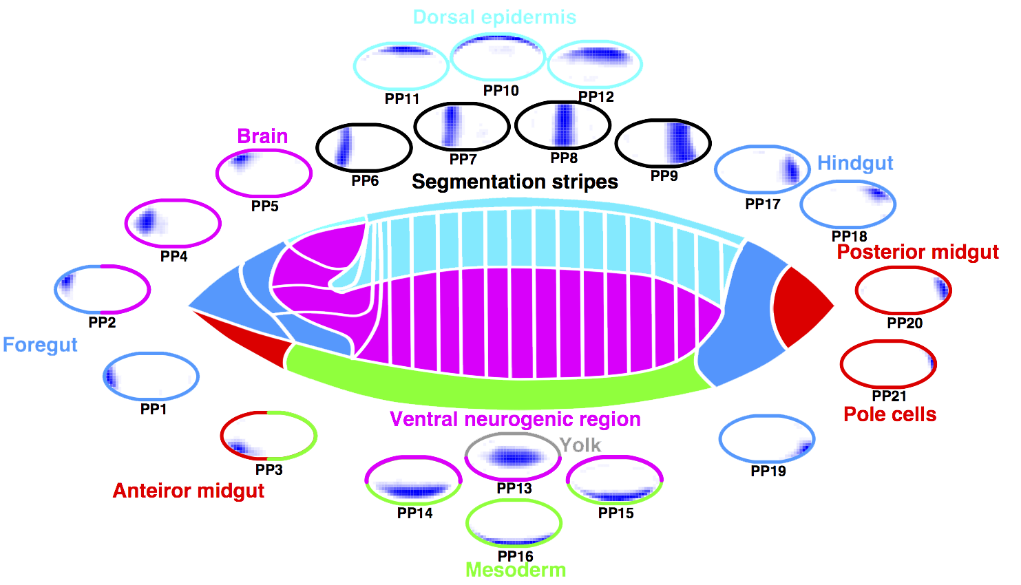
Berkeley Drosophila Genome Project:
TF spatial gene expression patterns
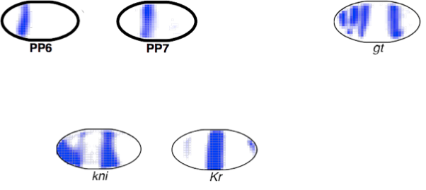
Pre-organ region principal patterns (PP)
Wu et al. (2016)
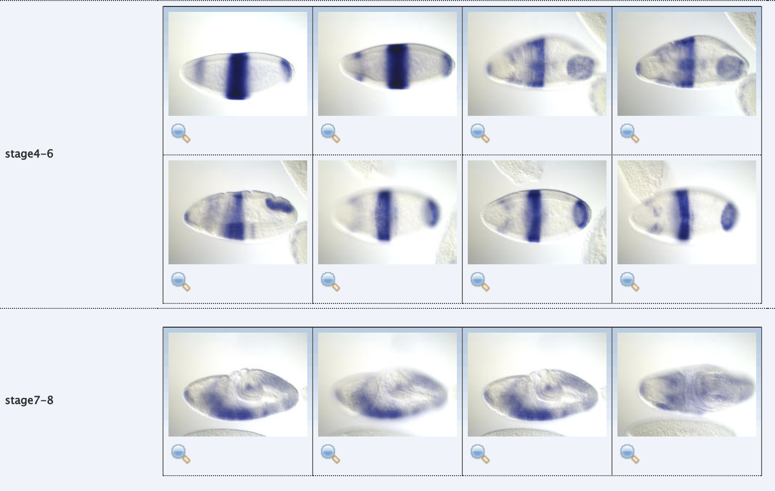
Predicting spatial gene expression patterns in early stage Drosophila embryos

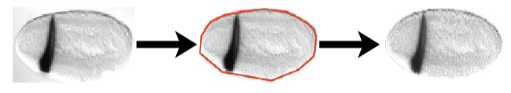
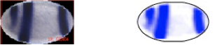
Detection and registration
Registered
images
Stain
extraction
Data: Wu et al. (2016)
- 405 pixels (~7 cells)
- : 22 TF gene expression patterns
- : 5 anterior-posterior PPs
Principal patterns (PP)
From genomic to statistical interactions: spatial expression
activators
repressors
PP7 expression rule
Region of the embryo
Expression levels of p transcription factors (TFs)
Test case: the gap gene network


Fruitfly embryo segmentation
Human embryo segmentation
Nobel Prize in Physiology or Medicine 1995
Edward B. Lewis, Christiane Nusslein-Volhard, Eric F. Wieschaus
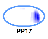
Predicting spatial gene expression patterns in early stage Drosophila embryos
: interactions correctly predicted
: interactions missed
PP17 interactions
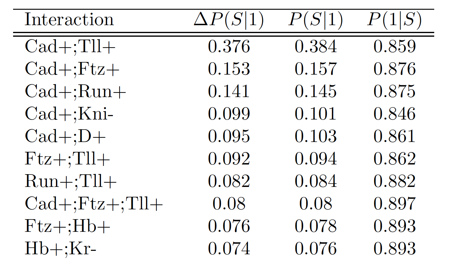

Cad
Tll
Ftz
Interactions recovered in spatial expression data co-bind at enhancer elements
Blimp-1
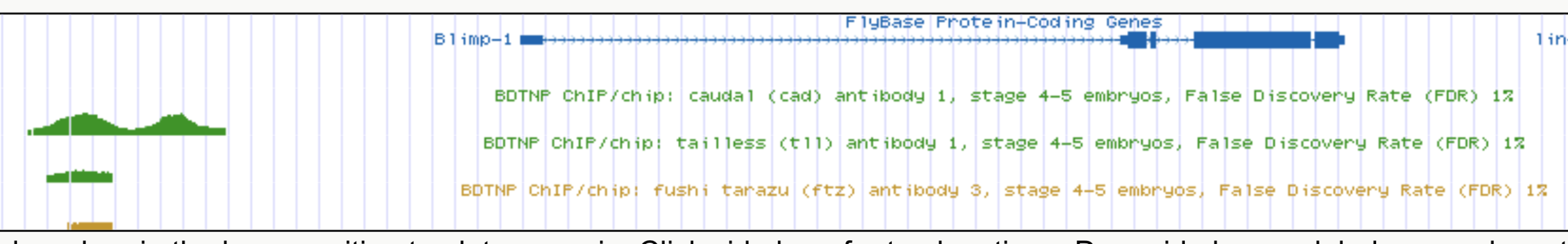
Cad
Tll
Ftz
Cad, Tll, Ftz
binding
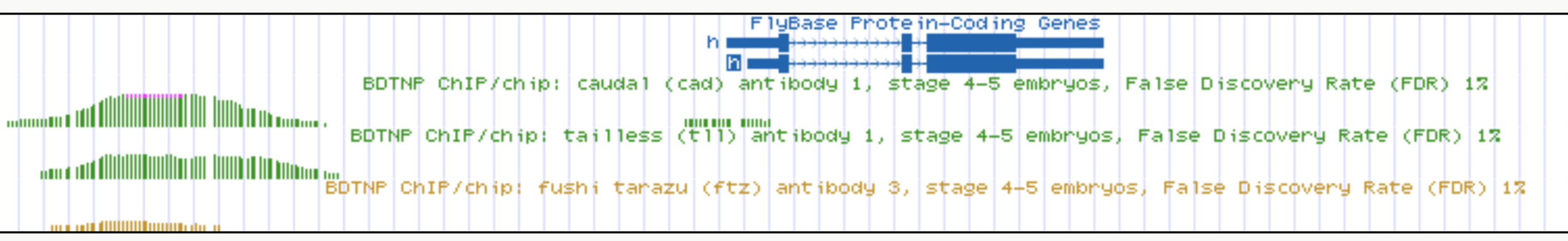
Interactions recovered in spatial expression data co-bind at enhancer elements
h
Cad
Tll
Ftz
Cad, Tll, Ftz
binding
Summary
- iRF and s-iRF identify well known interactions in Drosophila and posit new, high-order interactions surrounding important regulatory factors in the early embryo.
- By decoupling interaction order from the computational cost of discovery, iRF and s-iRF allow us to investigate mechanisms in genome biology and beyond (King et al., 2018; Long et al. 2018)
Other PhD projects
- PCS inference for ML models/algorithms
Joint with: Bin Yu
- Decoding spatial gene expression patterns in late stage Drosophila embryos
Joint with: Runjing Liu, Erwin Frise, Susan Celniker, Bin Yu
- Evaluating interpretability in ML models/algorithms
Joint with: Reza Abbasi Asl, Jamie Murdoch, Chandan Singh, and Bin Yu
Future work
- Investigating and characterizing emergent phenomena in biological systems, with a focus on disease states (e.g. neurodegeneration)
- Extracting localized interactions from ML models
- Incorporating dependencies into ML models
- Building mechanistic constraints/experimental results into ML models
- Characterizing mechanisms in heterogeneous cell populations
- Capturing dynamics of cellular behavior/responses
- Exploring how mechanistic insights inform treatment strategies
Biological challenges
Statistical challenges
Ackowledgements


S. Basu
J. Brown
B. Yu
S. Celniker
E. Frise