MAKE NEW TITLE
PGA: Plane-Based Geometric Algebra \(\mathbb{ R}^{d,0,1}\)
Leo Dorst
l.dorst@uva.nl
Steven De Keninck
enkimute@gmail.com

Contents (ADAPT)
- Plane-based: it's all done with mirrors
- The algebra of multiple reflections
- Specification by invariants
- Objects and operators unified
PGA: Why, What's New?
- Bullet One
- Bullet Two
- Bullet Three
It's All Done with Mirrors
- Bullet One
- Bullet Two
- Bullet Three

Plane Reflection Algebra
Define a sensible geometric product such that reflection becomes:
The mirror plane reflects to its negative:
\[a \mapsto -a\,a\,a^{-1} = -a\]
So planes are oriented, they have sides.
To make the geometric product work in the right way, it needs to be bilinear, associative, not generally commutative, and square to a scalar (which is \(a^2 = a \cdot a\) ).
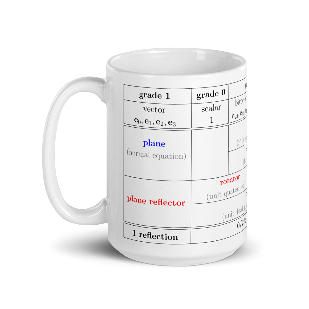
A Plane is a PGA Vector
You may have used the homogeneous coordinates, \(\[vec{n},-\delta]\) for a plane.
In PGA we use:
$$p = \mathbf{n} + \delta\,{\sf e}.$$
Here \({\sf e}\) is a basis vector for the extra dimension.
It can be interpreted as the plane at infinity and satisfies \[{\sf e}^2 = 0\]
Commutation and Perpendicularity
A plane \(b\) perpendicular to a mirror \(a\) reflects to itself: \( -a \,b \, a^{-1} = b\). So we have:
algebra \(\rightarrow\) \(a \,b = - b \, a \Longleftrightarrow b \, \bot a\) \(\leftarrow\) geometry
perpendicular planes anticommute
This holds especially for the Euclidean coordinate planes:
\(e_1\,e_2 = -e_2 \, e_1\) etc.
We also demand it for the special plane \(\mathsf{e}\): \(e_i \, \mathsf{e} = -\mathsf{e}\, e_i\).
Of course, parallel planes commute: \(e_i \, e_i = e_i \, e_i \).
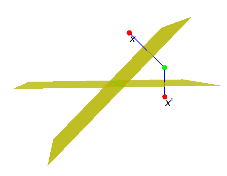
Multiple Reflections Give Operator Elements
Perform two reflections in succession:
\(x ~~~\mapsto~~-a_2 \, (-a_1\, x \,a_1^{-1})\, a_2^{-1}= (a_2\,a_1)\, x\, (a_2\,a_1)^{-1}\)
This shows that elements of the form \((a_2\,a_1)\) act as rotation/translation operators. We can clearly continue this with more reflections.
A geometric product of planes produces a motion, when applied as sandwiching. We call it a motor.
Motors are computational elements of the plane-based geometric algebra PGA: Euclidean motion operators are thus naturally included!
Parallel Reflections: Translation Operators
Double reflection in two parallel planes:
\(p_2\,p_1 =\) \((\mathbf{n} + \delta_2 \mathsf{e}) \, (\mathbf{n} + \delta_1 \mathsf{e}) \)
\(= \mathbf{n}\,\mathbf{n} + \delta_2\, \mathsf{e} \,\mathbf{n} + \delta_1\,\mathbf{n}\,\mathsf{e} + \delta_2\delta_1 \,\mathsf{e}\,\mathbf{n}\,\mathsf{e}\,\mathbf{n} \)
\(= 1 + (\delta_2-\delta_1) \mathbf{n} \, \mathsf{e} + 0\)
\(= 1 + \mathbf{t} \mathsf{e}/2\)
\(= 1- \mathsf{e} \,\mathbf{t}/2 + \frac{1}{2!}(-\mathsf{e} \,\mathbf{t}/2)^2+\cdots\)
\(= e^{-\mathsf{e} \,\mathbf{t}/2}\)
Translations are additive:
\((1+\mathbf{t}_2\mathsf{e}/2)\,(1+\mathbf{t}_1\mathsf{e}/2)\) \( = 1 + (\mathbf{t}_2+\mathbf{t}_1)\mathsf{e}/2 + \mathbf{t}_2\mathsf{e}\,\mathbf{t}_1\mathsf{e}/4\) \(= 1 +(\mathbf{t}_2+\mathbf{t}_1)\,\mathsf{e}/2\)
You see how \({\sf e}^2 = 0\) is crucial to making this work.
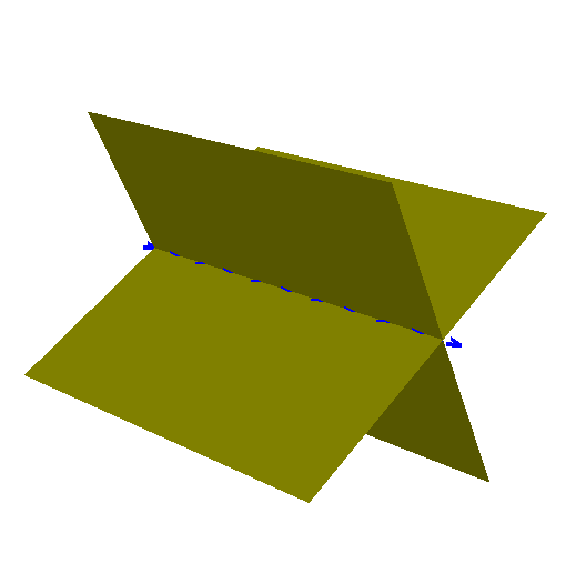
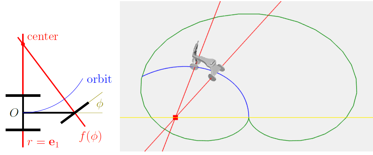
Tilted Plane Reflections: Rotation Operators
Let us choose handy local coordinates so that the two planes are \(p_1= e_1\), and \(p_2 = e_1 \cos\phi' + e_2\sin\phi'\). Then
\(p_2\, p_1 =\) \((e_1 \cos\phi' + e_2\sin\phi')\,e_1\)
\(= e_1^2 \cos\phi' + e_2e_1\,\sin\phi'\)
\(= \cos\phi' - L \sin\phi' \)
\(= e^{-L\phi/2}\)
with \(e_1e_2 =\)\( L\) the common line and \(\phi\) the rotation angle.
Note that a line has a negative square:
\(L^2 = e_1e_2e_1e_2 = - e_1^2e_2^2 = -1\),
motivating the exponential notation.
The Line Common to Two Planes Is a Bivector
The line common to two planes \(a\) and \(b\) is the element
\(L = a \wedge b = \frac{1}{2} (a \, b - b\, a)\).
It is not normalized, but the norm \(|L| = \sin(\angle(a,b))\) is a useful numerical quantity.
Element \(a \wedge b\) is called a bivector or 2-vector.
The wedge product \(\wedge\) (also known as the meet or outer product) is bilinear, anti-symmetric, and extended to be associative. Note that \(a \wedge a = 0\).
(Associativity by defining \(x \wedge A = \frac{1}{2}(x \, A + \hat{A}\,x)\), with \(\hat{A}\) giving minus sign for odd \(A\) ).
Bonus Material:
The Line Is Indeed Invariant Under Rotation
The element \(a \wedge b\) commutes with the rotation operator \(a \, b\).
\( (a \wedge b)\, (a\,b) = \frac{1}{2} (a \, b \, a \, b - b\,a\,a\,b) \)
\(= \frac{1}{2} (a \, b \, a \, b - 1) \)
\(= \frac{1}{2} (a \, b \, a \, b - a\,b\, b\,a)\)
\(= (a \, b) \, (a \wedge b) \)
Therefore, the element \(L = a \wedge b\) is invariant under the rotation \(R_{L\phi} =a \, b\), for
\( R_{L\phi}\, L \,R^{-1}_{L\phi} = L\, R_{L\phi}\,R^{-1}_{L\phi} = L\).
So it must be the common line. Circular reasoning is OK for rotations!
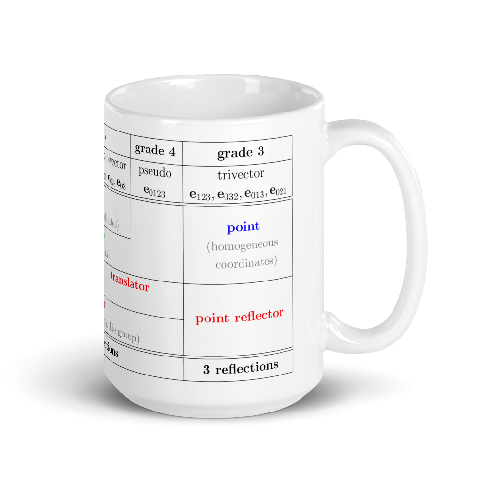
A Point: a Trivector Common to Three Planes
Standard example:
\( X \) \(= (e_1+x_1\mathsf{e}) \wedge (e_2+x_2\mathsf{e}) \wedge (e_3+x_3\mathsf{e})\)
\( = e_1e_2e_3 + x_1 \mathsf{e}e_2e_3 + x_2 \mathsf{e} e_3e_1 + x_3 \mathsf{e} e_1e_2\)
\( = e_1e_2e_3 - (x_1e_1 + x_2 e_2 + x_3e_3)\,\mathsf{e}e_1e_2e_3\)
\(= O - \mathbf{x} \, \mathcal{I}\)
Just like with homogeneous coordinates, a point \(X\) is characterized as \([1, x_1, x_2, x_3]\), but now on the PGA trivector basis \([e_1e_2e_3, -ee_2e_3, -ee_3e_1, -ee_1e_2]\).
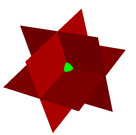
The trivector \(a \wedge b \wedge c\) is the point
common to three planes \(a, b, c\).
Operators and Objects
Only Axis and Angle Matter
REFER TO GAUGE FREEDOM, REPLAY DEMO?
DESIRE TO REPRESENT THAT WAY
TWO ISSUES: LINE REPR, AND EXP
Automatic Equivariance
SHOW PRINCIPLE
CONSEQUENCES:
THEORY - SIMPLE DERIVATIONS
PRACTICE - UNIVERSAL CODE IN TWO WAY: NOT JUST ANYWHERE, BUT ALSO ANYTHING
Exponential Representation of Motors
Just state it and the Log.
Wedge/Outer Product
Lorem ipsum dolor sit amet, consectetur adipiscing elit. Morbi nec metus justo. Aliquam erat volutpat.
3D Lines, 2D Points are Bivectors
Lorem ipsum dolor sit amet, consectetur adipiscing elit. Morbi nec metus justo. Aliquam erat volutpat.
3D Points are Trivectors
Lorem ipsum dolor sit amet, consectetur adipiscing elit. Morbi nec metus justo. Aliquam erat volutpat.
Decomposition of Motions
Chasles' Theorem & Lie Algebra
Lorem ipsum dolor sit amet, consectetur adipiscing elit. Morbi nec metus justo. Aliquam erat volutpat.
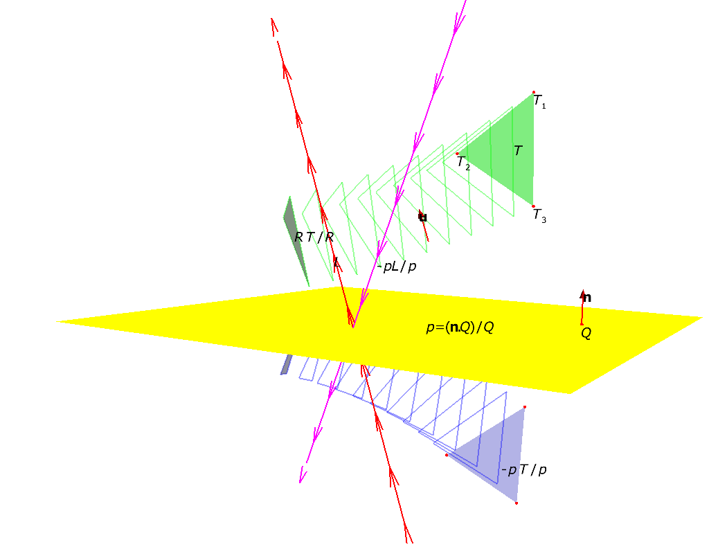
Projections
The Other Part of the Geometric Product
Lorem ipsum dolor sit amet, consectetur adipiscing elit. Morbi nec metus justo. Aliquam erat volutpat.
All Things Project Alike
Lorem ipsum dolor sit amet, consectetur adipiscing elit. Morbi nec metus justo. Aliquam erat volutpat.
General Linear Transformations: No Matrices Please
Lorem ipsum dolor sit amet, consectetur adipiscing elit. Morbi nec metus justo. Aliquam erat volutpat.
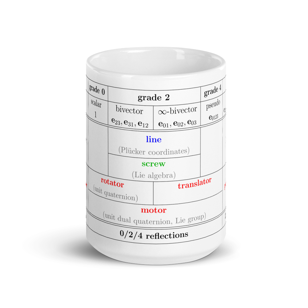
Ganja Coffeeshop Time!
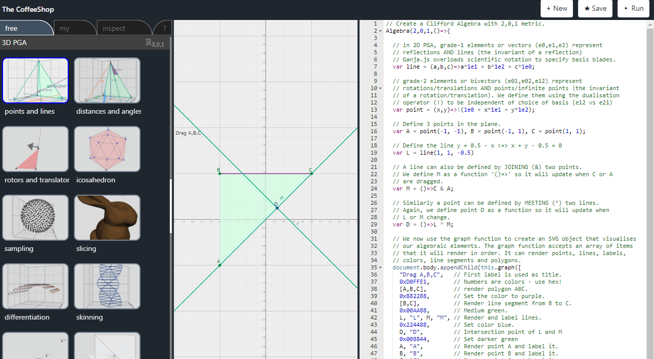
For all your Geometric Products, visit
Newtonian Dynamics in PGA
Leo Dorst
l.dorst@uva.nl
Steven De Keninck
enkimute@gmail.com
Overview
- Two Types of Lines
- Momentum and Inertia
- May the Forque Be with You
- Differentiating Motors
- Unified Dynamics
- Classical Mechanics Embedded
- Demos

Kinematics and Dynamics in PGA
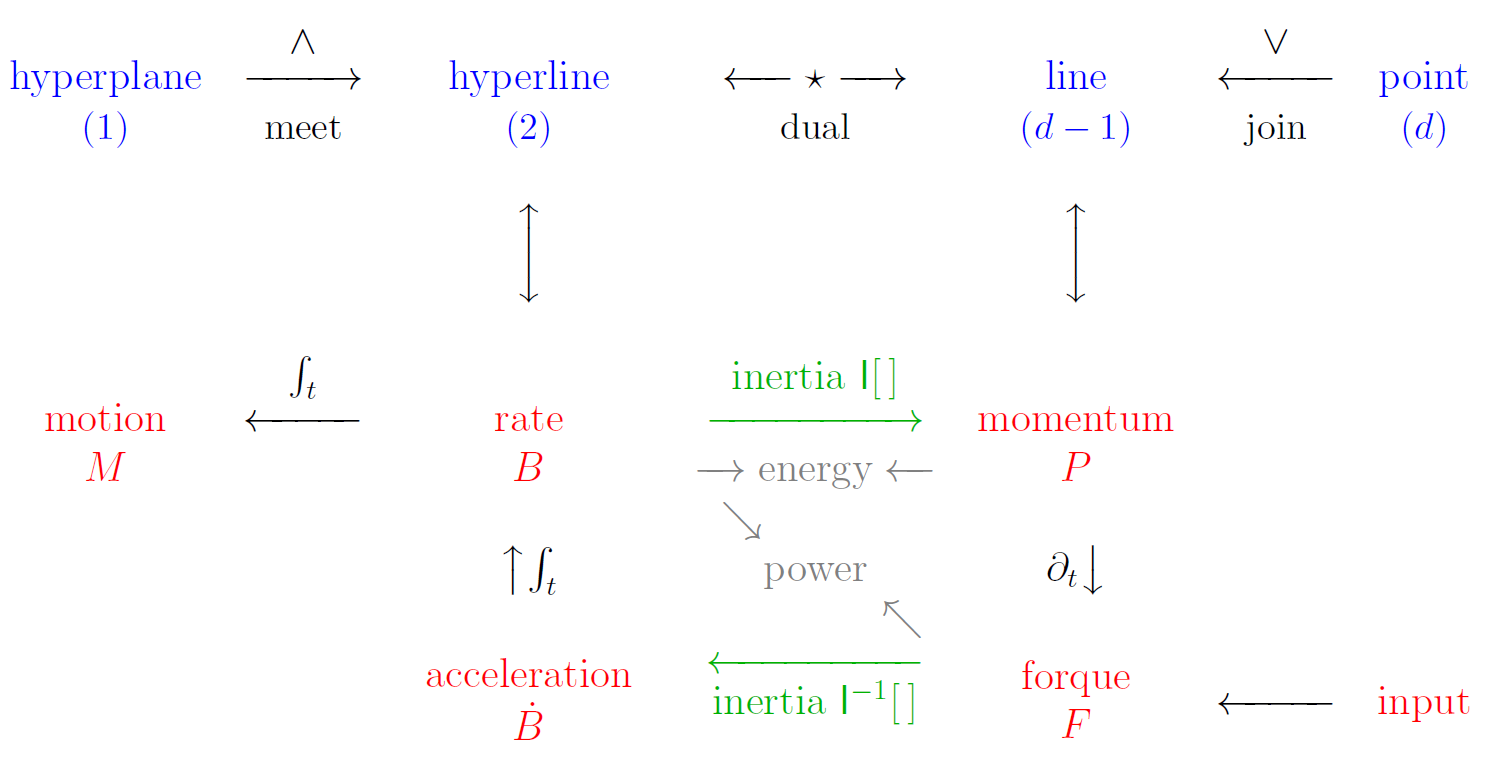
Kinematics and Dynamics in PGA
1. Join Lines
0. Kinematics
2. Mass in Motion
3. Forque Action
4. Derivatives
5. Dynamics
1. Two Types of Lines
Two planes meet in a line.
Two points join to form a line.
Are those lines the same type? No!
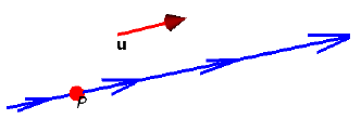
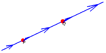
Points Move Along Lines
The line from point \(A\) to point \(B\) is the PGA element \[A \vee B \]
It is defined using the JOIN product \(\vee\), which is (in a Hodge sense) dual to the MEET \(\wedge\) (and, like it, a linear combination of geometric products).
One can derive from this that the line from \(A\) in direction \({\bf v}\) is: \[ {\bf v} \cdot A\]
The join in \({\mathbb R}^{d,0,1}\) of two \(d\)-vector points is a \((d-1)\)-vector.
- (Join) lines in \(d\)-D are \((d-1)\)-vectors!
- (Meet) hyperlines are 2-vectors in any dimension.
Consider a 2D picture of a tricycle in a plane, made of points and lines. Analyze and program up, then pop up the third dimension.
Some points remain points (2-vectors to 3-vectors), but the turning points become extruded to axis lines; they were 2D hyperlines.
Some lines remain lines (they were join lines), but the boundary lines become planes (they were 2D hyperplanes).
We need them all!
PGA encodes them all properly, so they extrude correctly to \(d\)-D.
Hyperlines vs Lines
2. Momentum and Inertia

The Momentum of a Moving Mass is a Line
A point with mass \(m\) moving with velocity \({\bf v}\) through a point \(X\) has as momentum \(P\) the join line:
\[ P=m\,X\vee (X-{\bf v}\mathcal{I})=m\,{\bf v}\cdot X\]
Note that the inclusion of the point \(X\), where things happen, is more specific than in Classical Mechanics (CM).
It is precisely this practice that makes the PGA momentum into an element of geometry, which allows PGA to be coordinate-free.
Inertial Momentum of a Point Cloud
We defined the linear inertia map \(I[\,]\), taking a 2-vector and producing a \((d-1)\)-vector. It contains all required information on the mass distribution.
PGA inertia is additive: it can be evaluated anywhere. Inertia of union is sum of inertias. No parallel axis theorem needed!
definition join line
moving by motor: bivector
defining inertia map
Masses Provide the Duality Map
to Convert Rates to Momenta
Rate \(B\) is for kinematics.
Momentum \(P\) is for dynamics.
Inertia \(I[\,]\) couples them.
momentum \(P\)
join line
\((d-1)\)-vector
rate \(B\)
hyperline
2-vector
inertia \(I[\,]\)
duality map
The PGA Inertia Map is not Symmetric
On a basis of principal frame bivectors \((e_{23},e_{31},e_{12},e_{01},e_{02},e_{03})\), the 3DPGA inertia map acts like the matrix:
Note the dual nature: converts Euclidean to ideal and vice versa.
In 2D, also from hyperlines \((e_{12},e_{01},e_{02})\) to lines \((e_0, e_2, e_1)\), it is:
classical mechanics inertia matrix
3.
May the Forque Be with You

A Force is a Line
Classically, you speak of a force vector \({\bf f}\) attached at a location \(X\), but ultimately only compute with \({\bf f}\) (and leave \(X\) in the text).
In PGA, we compute with the
force line \(F = {\bf f}\cdot\!X\)
This is a geometric object, free from convention on origin or choice of coordinates.
What does that mean, and why does it help enormously?
A Force Line Induces Torque Elsewhere
In PGA, we compute with the force line \(F = {\bf f}\cdot\!X\).
Consider the same force line \(F\) from another point \(Y\):
\(F = {\mathbf f} \cdot X = {\mathbf f} \cdot (O - \mathbf{x} \, \mathcal{I})\)
\(= {\mathbf f} \cdot (O - \mathbf{y} \, \mathcal{I}) + {\mathbf f} \cdot \big( (\mathbf{y}-\mathbf{x}) \, \mathcal{I} \big) \)
\( = {\mathbf f} \cdot Y + \big((\mathbf{y}-\mathbf{x}) \times {\mathbf f}\big) \wedge\mathsf{e}\)
force at \(Y\) torque at \(Y\)
Force and torque are unified in \(F\), how you experience them depends on where you are. No need for parallel axis theorem!
Let us call this element of physical geometry: forque.
(Yes, \(F\) is like a wrench from screw theory)
Momentum and Forques: Both Screw Lines
With both total momentum and total forque in the same format of \((d-1)\)-vectors, we are ready to work with Newton/Euler in a geometric, coordinate-free way, in any dimension.
There is a slight (and necessary) subtlety: a sum of lines is not a line but a screw line.
HARD TO DO COMPACTLY, JUST MENTION IT?
OR IS IT ALREADY IN THE PREVIOUS TALK
4. Differentiating Motors
Motors in World Frame or Body Frame
We can represent a given motor \(M\) (with initial state \(M_0\)) either in a world frame:
\(M\) = \(e^{-B_wt/2}\) \(M_0\),
or in the body frame:
\(M\) = \(M_0\) \(e^{-B_bt/2}\).
We then get a left or right bivector differential equation for \(M\):
\(\dot{M}\) = \(-\frac{1}{2} B_w M\) = \(-\frac{1}{2} M B_b\).
Either can be used to solve \(M\), it is a choice of convenience.
Differentiating a Moving Element
When an element is moved with a time-dependent motor \(M(t) = e^{-B t/2}\), we have
\(\partial_t X(t)\) \( = \partial_t (M(t) X_0 M(t)^{-1}) \)
\(= - \frac{B}{2} \, X(t) + X(t) \, \frac{B}{2}\)
\(= X(t) \times B\),
employing the commutator product: \(A \times B \equiv \frac{1}{2}(A\,B-B\,A).\)
Differential motions are thus determined by commutators with the bivectors of their motors.
This incorporates the Lie algebra of motions into GA.
Coupling Forque to Motion
Finally, some physics! Newton/Euler states that
the total forque gives the change of total momentum:
\[F = \dot{P}\]
and this fully determines the motion.
We thus need the time derivative of the momentum:
\[ \dot{P} = \partial_t {I}[B] = I[B] \times\!B + I[\dot{B}]\]
Masses move by \(M\), so inertia changes by \(\times B\) ...
... but \(B\) changes also.
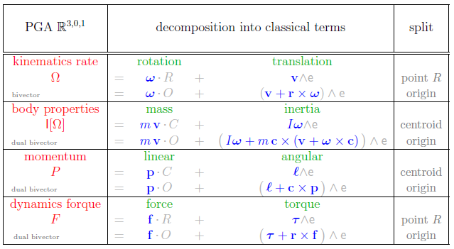
5. Unified Dynamics
Done: All in One
From \(F = \dot{P} = \partial_t {I}[B] = I[B] \times B + I[\dot{B}]\) and the motor equation, we have (in the body frame):
This is all of Newton/Euler dynamics, both linear and angular.
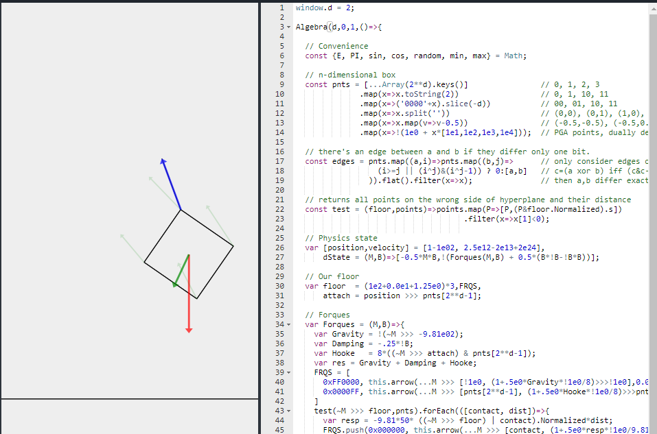
These equations can easily be integrated by numeric methods (and in some situations by hand).

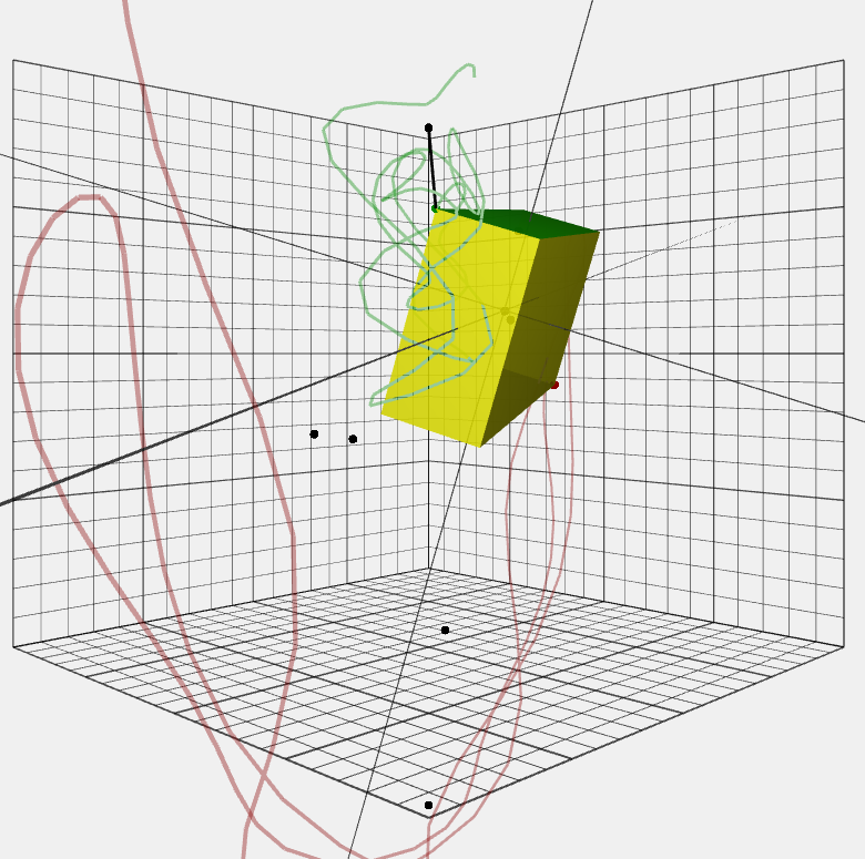
INSERT SOME DEMOS HERE
Kinematics and Dynamics in PGA
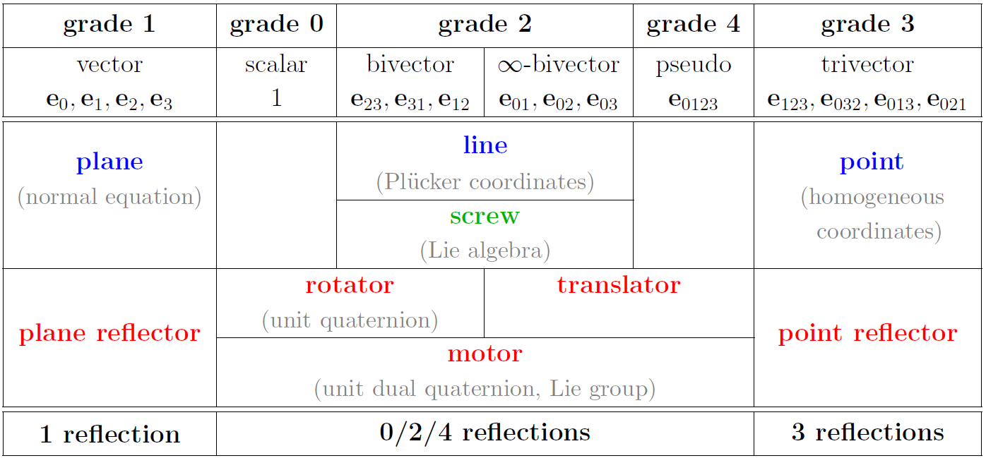
Elements of 3D PGA
In 3D lines and hyperlines look very similar, in coordinates.
This confusion held back integrated CM representation.
Screw Theory & Spatial Vectors
However:
- Neither employ bivectors, which complicates their math (some special products, in two dual spaces).
- Neither contain geometric elements, to act on directly.
- Perhaps because of that, they have remained specialized skills for too many years.
- They are specific for 3D; we know it's just as easy to be \(d\)-D.
There are two other 6D frameworks also combining linear and angular aspects for 3D, both also correct:
- screw theory (Ball, Study, 19th century)
- spatial algebra (Featherstone, 20th century)
6. PGA Embedding of 3D Classical Mechanics
Summary: Two for the Price of One
- PGA needs only 4 quantities to do all, CM takes 8
- PGA is coordinate-free: no descriptive basis needed
- CM is a pre-split version of PGA, hiding the location
- Conversion: name location \(.X\), use infinity \(\wedge {\sf e}\), simply add.

7. Ganja Coffeeshop Time!
For all your Geometric Products, visit