

2
1

Learning sparse features can lead to overfitting in neural networks
Leonardo Petrini,* Francesco Cagnetta,* Eric Vanden-Eijnden, Matthieu Wyart
1
1
2
1
Learning in high dimensions with neural nets
- Intuition: deep nets are able to solve high-dimensional tasks by learning relevant and low-dimensional features of the data
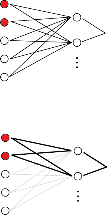
- Theory: learning sparse features beneficial for FCNs when task depend on few variables, \(f^*(x_1\dots, x_5) = f^*(x_1, x_2) \)
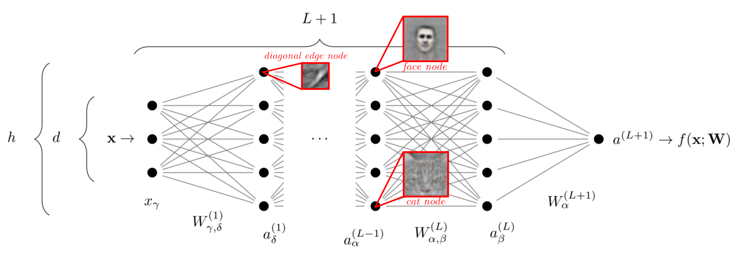
initialization (dense)
trained (sparse)

Drawbacks of learning features
-
Evidence: on images, feature learning in FCNs and for gradient descent is outperformed by the corresponding kernel method.
-
Hypothesis:
- image classes vary smoothly along small deformations;
- high smoothness requires a continuous distribution of neurons;

Geiger et al. (2020a,b); Lee et al. (2020)
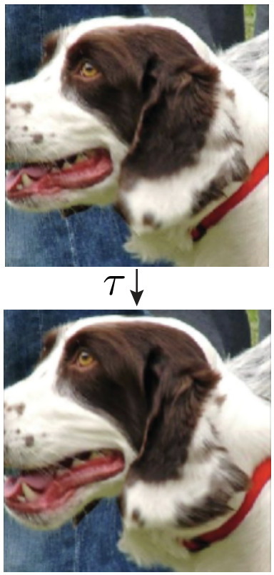

Figure. Kernel predictor is smoother along diffeomorphisms for image classification.
more smooth
Supervised regression on the sphere
Task: regression with \(n\) training points \(\{\bm x\}_{i=1}^n\) uniformly sampled from the hyper-sphere \(\mathbb{S}^{d-1}\) and target function of controlled smoothness \(\nu_t\):
$$\| f^*(\bm{x})-f^*(\bm{y})\| \sim \|\bm{x}-\bm{y}\|^{\nu_t} $$
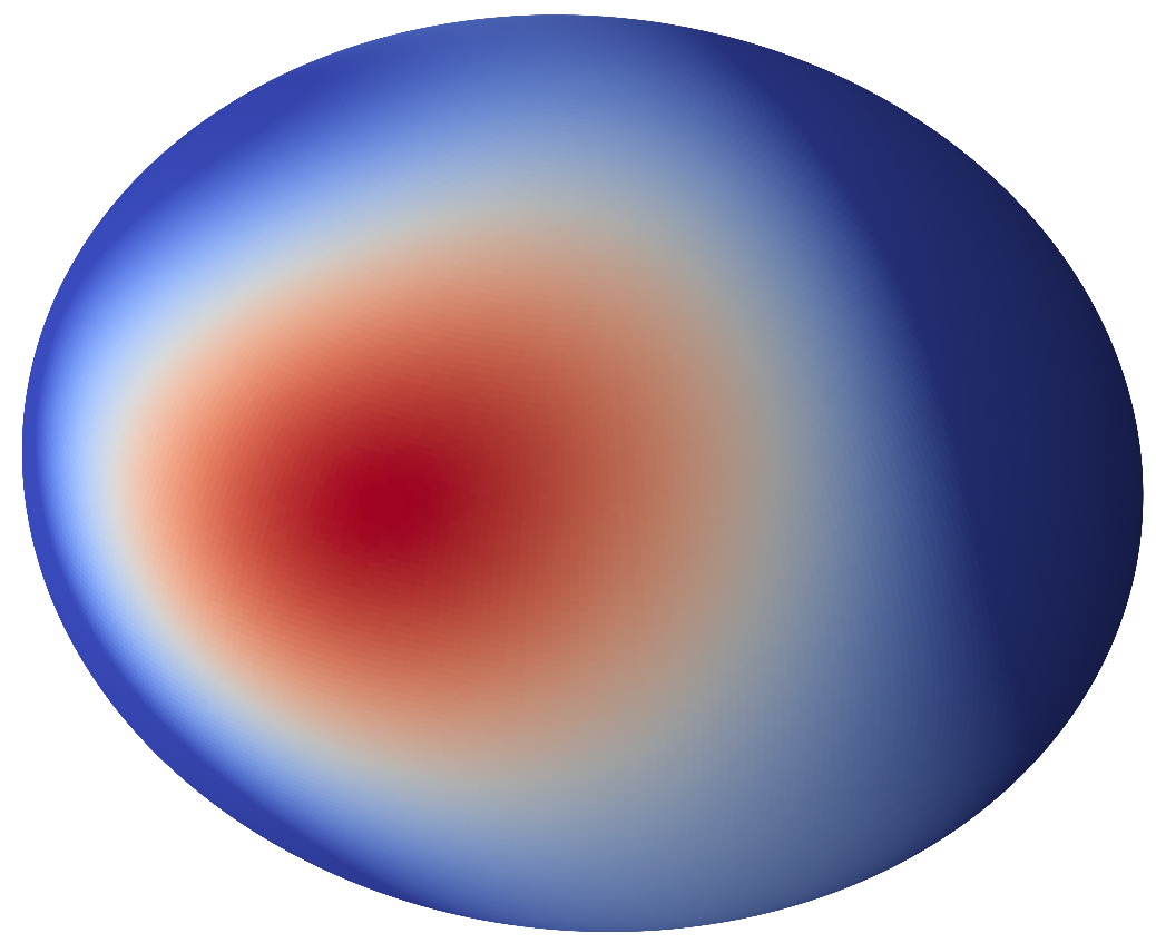
High smoothness
(large \(\nu_t\))
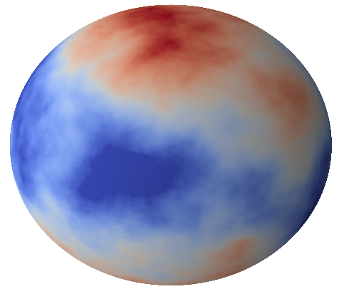
Low smoothness
(small \(\nu_t\))
log test error
log train set size
log test error
log train set size
feature learning
kernel regime
Training regimes and sparsity
Architecture: one-hidden-layer fully-connected with ReLU activations,$$f(\bm{x}) = \frac{1}{\mathcal{N}} \sum_{h=1}^H w_h \sigma( \bm{\theta}_h\cdot\bm{x}) $$
\(H\to\infty\): the choice of the normalization constant \(\mathcal{N}\) controls the training regime, $$\qquad\qquad\mathcal{N} = H \qquad \qquad \qquad\qquad\qquad\qquad\qquad \mathcal{N} = \sqrt{H}$$
feature learning
kernel regime

Jacot et al. (2018);
Bach (2018); Mei et al. (2018);
Rotskoff, Vanden-Eijnden (2018)...
Training regimes and their predictors
Architecture: our aim is to approximate the target function by a one-hidden-layer neural network of width \(H\), $$f(\bm{x}) = \frac{1}{\mathcal{N}} \sum_{h=1}^H w_h \sigma( \bm{\theta}_h\cdot\bm{x}) $$
as \(H\to\infty\), the choice of the normalization constant \(\mathcal{N}\) controls the training regime, $$\qquad\qquad\mathcal{N} = H \qquad \qquad \qquad\qquad\qquad\qquad\qquad \mathcal{N} = \sqrt{H}$$
and the predictors take the forms:
feature learning
kernel regime

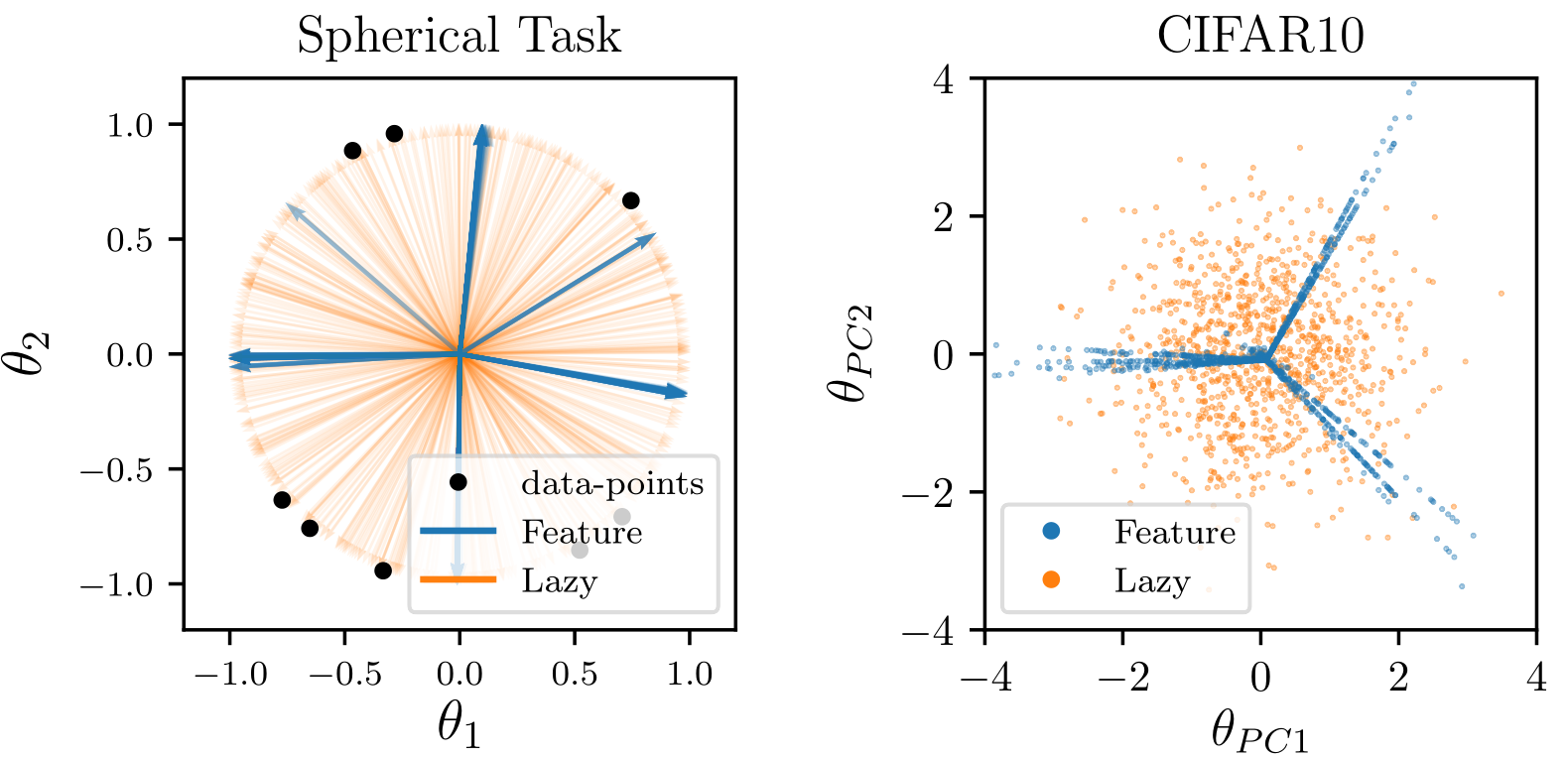
- First layer weights \(\bm \theta_h\) after training:
Generalization error in the two regimes
Atomic solution: the feature regime predictor takes the following form,$$f^{\text{FEATURE}}(\bm{x}) = \sum_{i=1}^{n_A} w^*_i \sigma( \bm{\theta}^*_i\cdot\bm{x}) , \quad n_A = O(n),$$
Kernel trick: while the kernel predictor can be written as (with \(K\) the NTK), $$f^{\text{LAZY}}(\bm{x}) =\sum_{i=1}^n g_i K(\bm{x}_i\cdot \bm{x}).$$
Boyer et al. (2019);
Notice that \(K\) is smoother than the ReLU function \(\sigma\), leading to a smoother predictor.
The scaling of generalization error is controlled by the smoothness of \( \sigma, \, K\):

predictor
target
predictor
training point
Conclusions and open questions
- Central result: learning features can be detrimental as it leads to a sparse representation not suited for all tasks, e.g. if target function varies smoothly along some directions in input space (for FCNs: rotations, translations, diffeomorphisms);
- Open question: what are the benefits of learning features in modern architectures?
Thank you.
- In passing we show how to compute the generalization error for one-hidden-layer FCNs based on the atomic solution of empirical risk minimization and relate it to the smoothness of the activation function;
end
The puzzling success of deep learning
- Deep learning is incredibly successful in wide variety of tasks
-
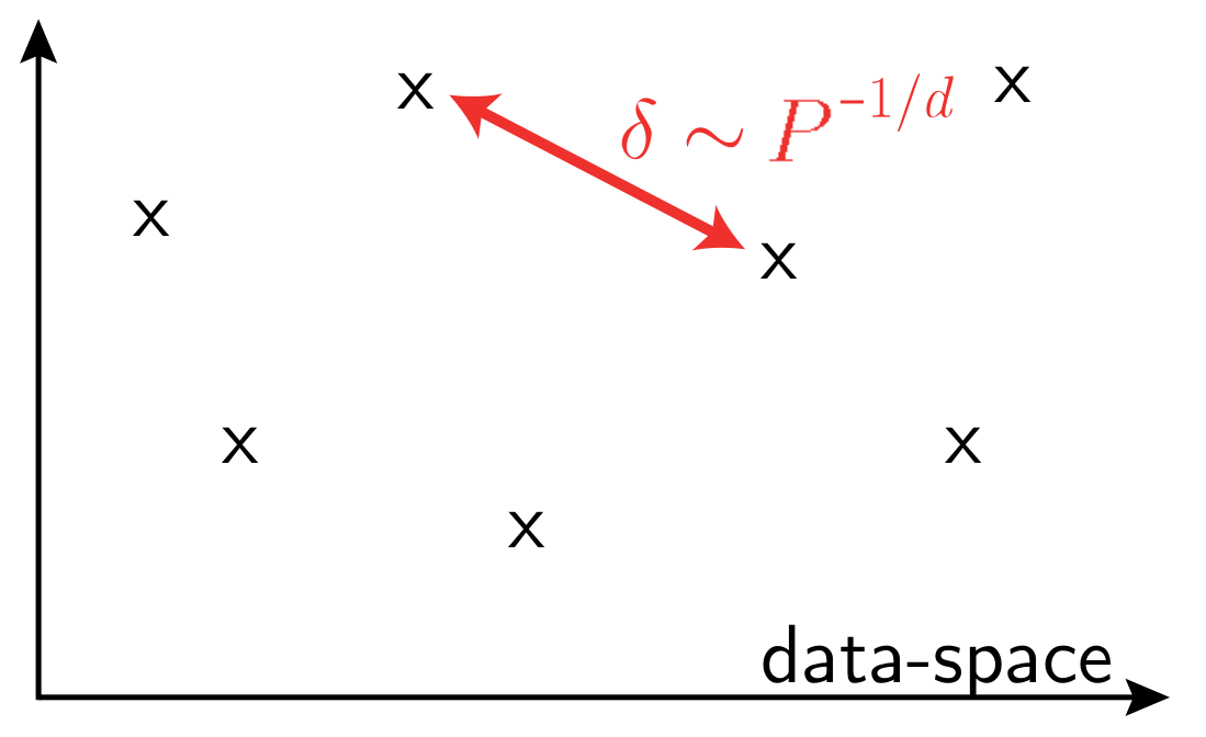
Curse of dimensionality when learning in high-dimension,
in a generic setting
vs.
- In high dimension, data that have little structure cannot be learned
\(P\): training set size
\(d\) data-space dimension
Is the secret of NNs in their ability to capture this structure?
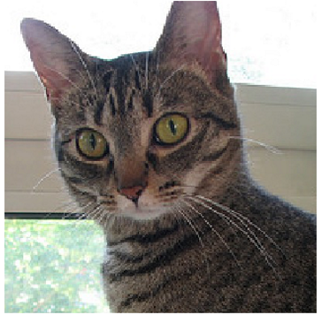
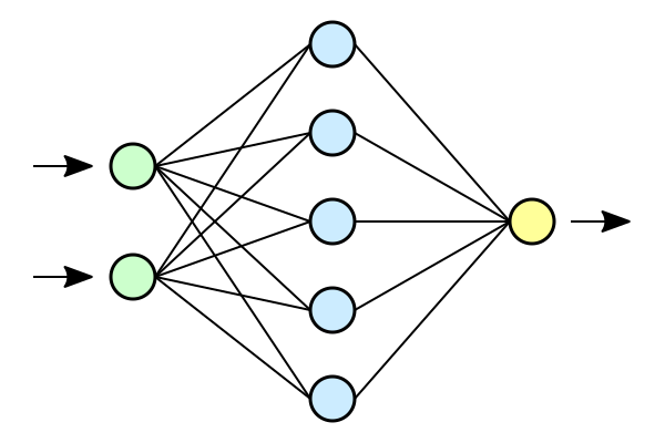
Cat
Learning features in neural networks (i)

The success of neural nets is often attributed to their ability to learn relevant features of the data
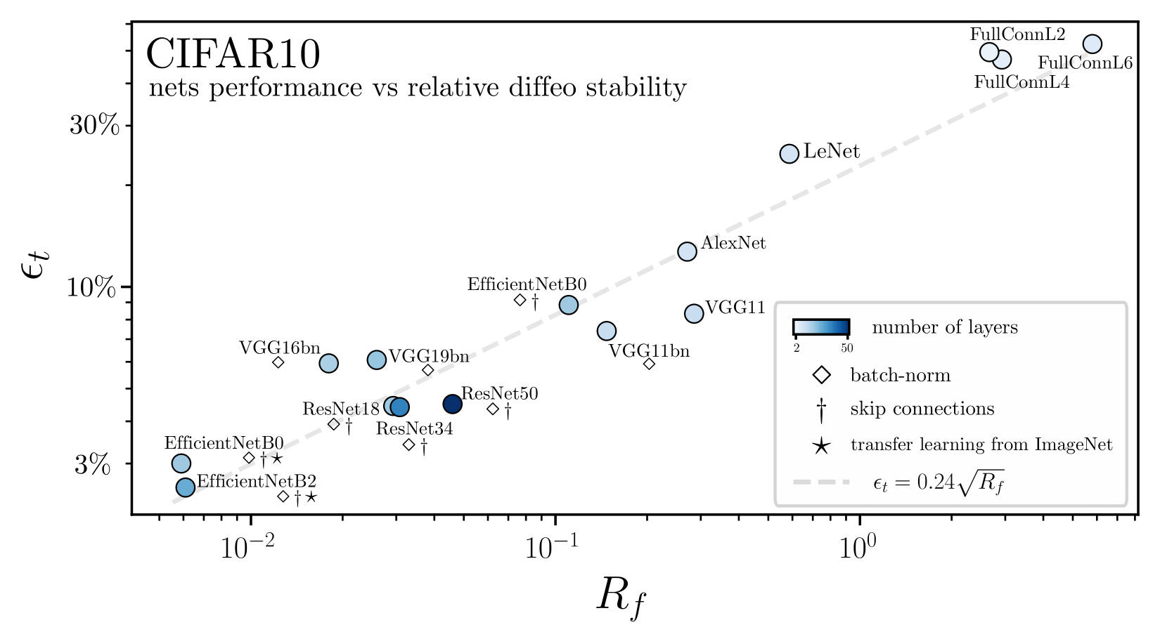
Still, this feature learning is not always beneficial. See for example the training of fully-connected nets on images:

Geiger et al. (2020a,b); Lee et al. (2020)
test error
deformation stability
[Petrini et al. 2021]
initialization


FCNs
Learning features in neural networks (ii)
Moreover, FCNs do not learn a meaningful representation of the data:
- Networks that perform well in the feature regime learn to become stable wrt input deformations;
- FCNs get worse, in this respect, when compared to initialization.

Perks and drawbacks of learning features in neural nets?
two training regimes exist, depending on the initialization scale
feature learning
(rich, hydrodynamic...)
neural representation evolves
Theory of infinite-width FCNs
lazy training
\(\sim\) kernel method
vs.
- Many examples exist where feature > lazy for FCNs;
- However, they all involve settings where the task depends on a few relevant directions of input space that are linear;
- This is (e.g.) the case of corner pixels in images;
- Still, it does not seem to play a prominent role in learning these data.
Jacot et al. (2018); Chizat et al. (2019); Bach (2018); Mei et al. (2018); Rotskoff, Vanden-Eijnden (2018)...
Bach (2017);
Chizat and Bach (2020); Ghorbani et al. (2019, 2020); Paccolat et al. (2020);
Refinetti et al. (2021);
Yehudai, Shamir (2019)...
How to rationalize the feature < lazy case?
e.g.
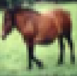
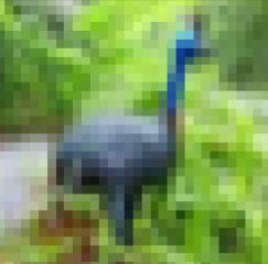
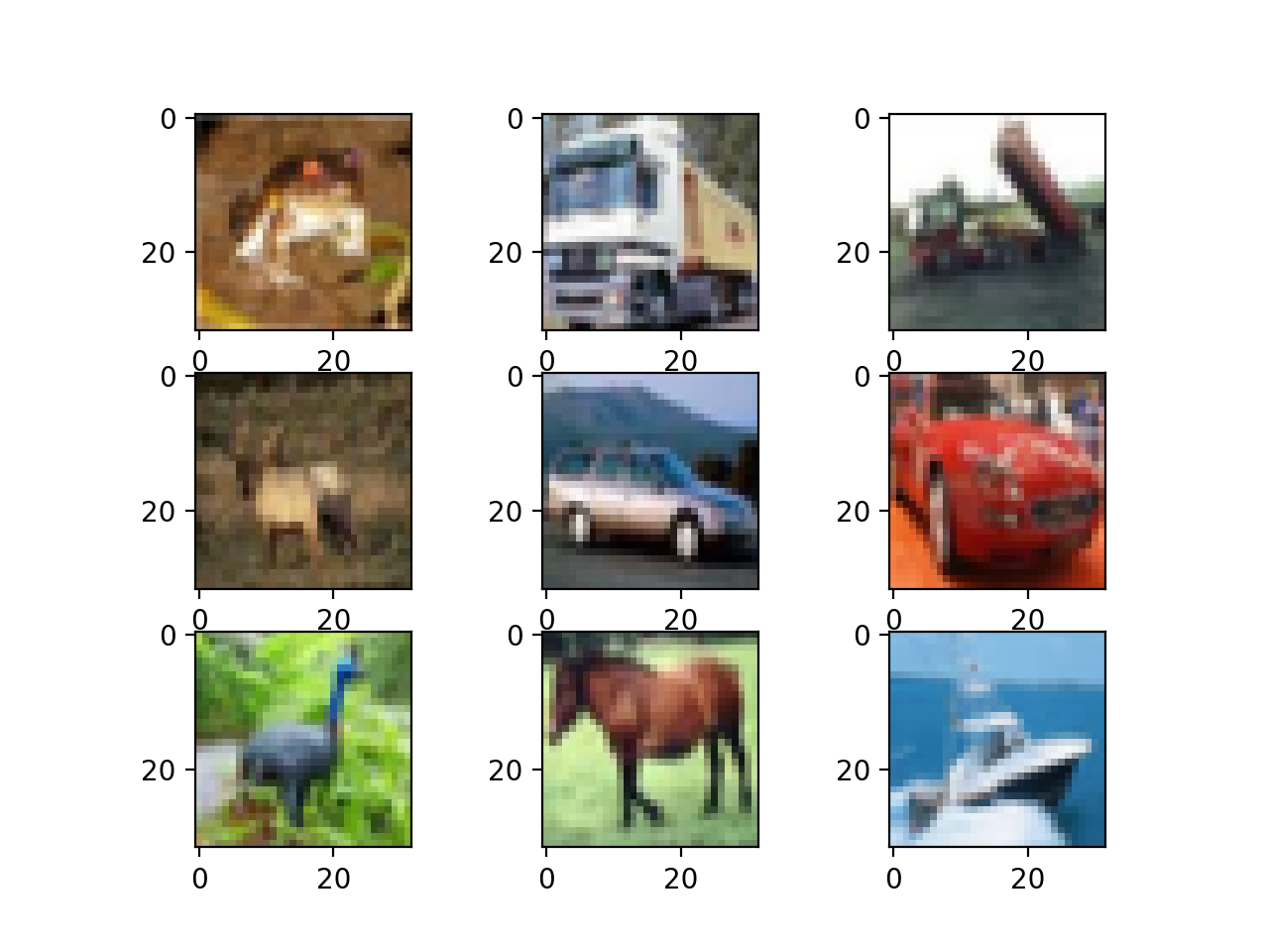
CIFAR10 data-point
- Feature learning can perform worse than lazy training as it leads to a sparse neural representation;
- Sparse representations are detrimental when the task is constant or smooth along some input-space directions;
- We illustrate this for
- regression of Gaussian random functions on the d-sphere
- benchmark image datasets
Our contribution:

deformation stability
[Petrini et al. 2021]

Random functions on the sphere
Task: regression with \(n\) training points \(\{\bm x\}_{i=1}^n\) uniformly sampled from the hyper-sphere \(\mathbb{S}^{d-1}\) and target a Gaussian random process
$$f^*(\bm x) = \sum_{k > 0} \sum_{l=1}^{\mathcal{N_{k, d}}} f_{k, l}^* Y_{k, l}(\bm x) \quad \text{with} \quad \mathbb{E}[{f^*_{k,l}}]=0,\quad \mathbb{E}[{f^*_{k,l}f^*_{k',l'}}] = c_k\delta_{k,k'}\delta_{l, l'},$$
with controlled power spectrum decay
$$c_k\sim k^{-2\nu_t -(d-1)} \quad \text{for}\quad k\gg 1.$$
This determines the target smoothness in real space
$$\mathbb{E}[{\vert f^*(\bm{x})-f^*(\bm{y})\rvert^2}]=O( |\bm{x}-\bm{y}|^{2\nu_t} )=O((1-\bm{x}\cdot\bm{y} )^{\nu_t} ) \quad\text{ as }\ \ \bm{x}\to\bm{y}.$$


spherical
harmonics
Neural Network and Training Regimes (i)
We consider a one-hidden-layer ReLU network of width \(H\), $$f^{\xi}_H(\bm{x}) = \frac{1}{H^{1-\xi/2}} \sum_{h=1}^H \left(w_h \sigma( \bm{\theta}_h\cdot\bm{x}) - \xi w_h^0 \sigma(\bm{\theta}_h^0\cdot \bm{x})\right),$$
where \(\xi\) controls the training regime such that we get well-defined \(H \to\infty\) limits:
-
Lazy regime \((\xi = 1)\). The network can be linearized around its initialization value and its behavior is fully determined by the Neural Tangent Kernel,
$$K_{NTK}(\bm x, \bm y) = \nabla_W f(\bm x) \nabla_W f(\bm y),$$
i.e. training corresponds to kernel regression with the NTK and the predictor takes the form $$ f^{\text{LAZY}}(\bm{x}) =\sum_{i=1}^n g_i K^{\text{NTK}}(\bm{x}_i\cdot \bm{x})\quad\text{ with } f^*(\bm{x}_j) =\sum_{i=1}^n g_i K^{\text{NTK}}(\bm{x}_i\cdot \bm{x}_j), \quad j=1,\ldots,n.$$
initialization
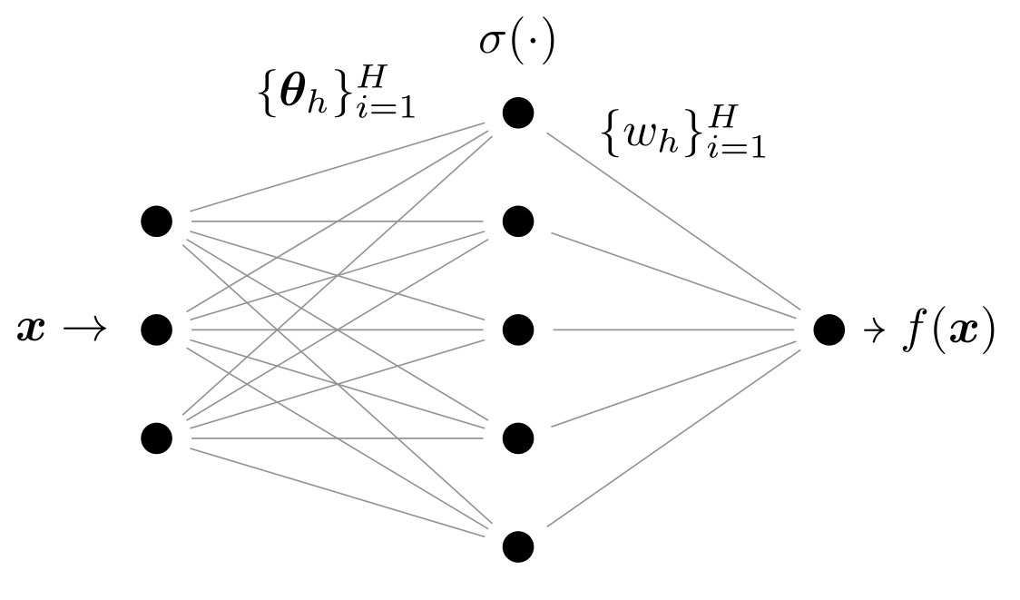
features
weights
ReLU
Neural Network and Training Regimes (ii)
- Feature regime \((\xi = 0)\). Here we get the so-called mean-field limit: $$\lim_{H\to\infty} f^{\xi=0}_H(\bm{x}) = \int_{\mathbb{S}^{d-1}} \sigma(\bm{\theta}\cdot\bm{x}) d\gamma(\bm{\theta}).$$ The optimal \(\gamma\) having minimal norm is then determined by $$\gamma^*= \argmin_{\gamma} \int_{\mathbb{S}^{d-1}} \lvert d\gamma(\bm{\theta})\rvert \quad \text{subject to} \quad \int_{\mathbb{S}^{d-1}} \,\sigma(\bm{\theta}\cdot\bm{x}_i)d\gamma(\bm{\theta}){=}f^*(\bm{x}_i)\quad \forall i=1,\dots,n. $$ Notice that this problem is equivalent to Lasso regression and hence the solution \(\gamma^*\) is unique and sparse (i.e. supported on a number of neurons \(n_A \leq n\) with probability 1. The predictor then reads $$ f^{\text{FEATURE}}(\bm x) = \sum_{i=1}^{n_A} w_i^* \sigma(\bm{\theta^*}_i\cdot \bm{x}).$$
Recall:
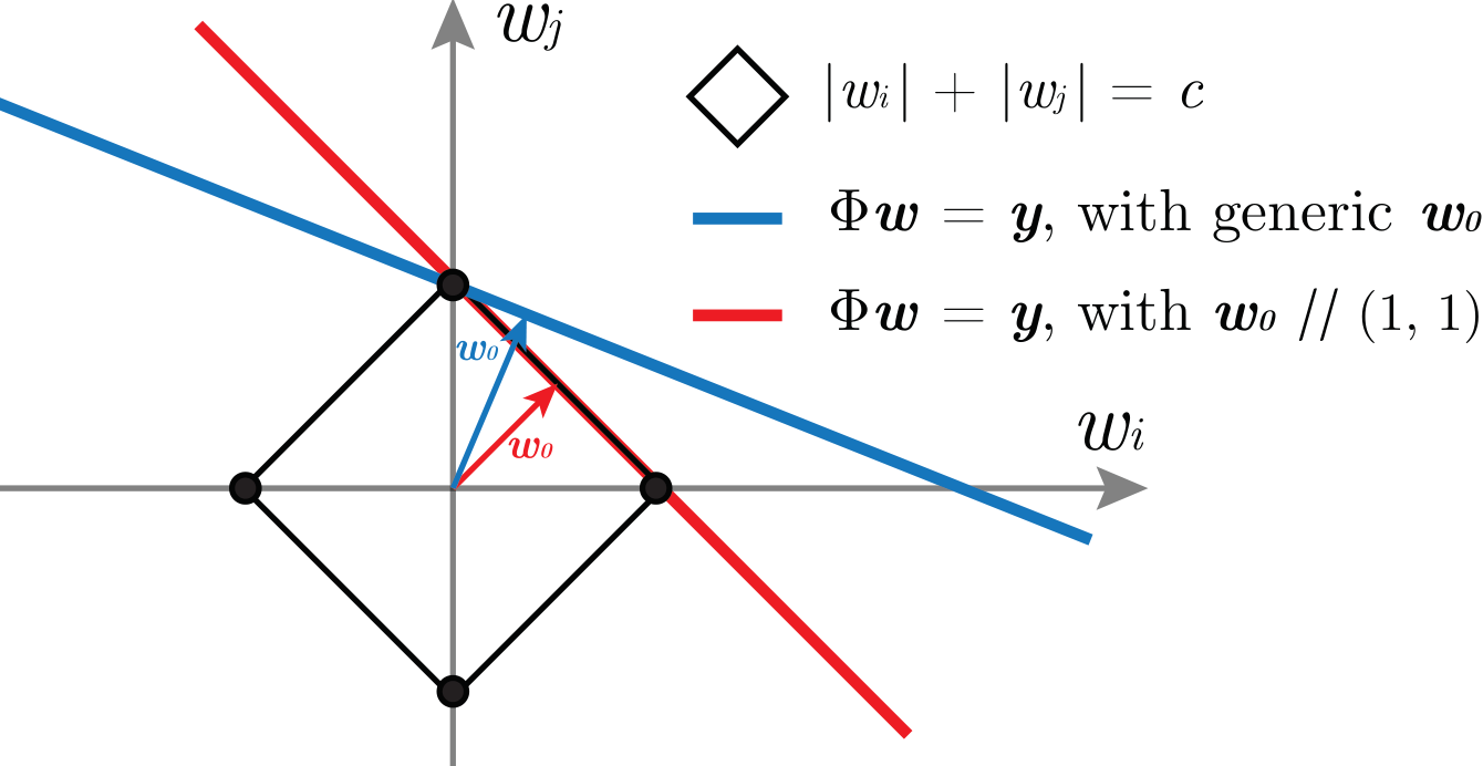
Lasso regression
Generalization error asymptotics (i)
The mean-square error measures the performance in both regimes: $$\epsilon(n) = \mathbb{E}_{f^*} \int_{\mathbb{S}^{d-1}} d\bm x \, ( f^n(\bm{x})-f^*(\bm{x}))^2 = \mathcal{A}_d n^{-\beta} + o(n^{-\beta}),$$ and we are interested in predicting the decay exponent \(\beta\) controlling the behavior at large \(n\). In both regimes, the predictor reads $$f^n(\bm{x}) = \sum_{j=1}^{{O}(n)} g_j \varphi(\bm{x}\cdot\bm{y}_j)\qquad\qquad\qquad\qquad\qquad\qquad\qquad\qquad$$
We first threat \(d=2\) and then generalize to any \(d\).
Recall:
Generalization error asymptotics (ii): \(d=2\)
In \(d=2\) (random functions on a circle), we can compute \(\beta\) as \(n\to\infty\) by:
- noticing that the predictor \(f^n(x) = \sum_j g_j \hat{\varphi}(x-x_j)\) has a number of cusps that is proportional to \(n\) and at average distance \(\delta \sim 1/n\);
-
as \(n\to\infty\), in between cusps, the predictor can be approximated by parabolas, with curvature controlled by the target function, then
- if the predictor is smooth enough (\(\nu_t > 2\)), then a Taylor expansion gives $$\epsilon(n) \sim \delta^4 \sim n^{-4},$$
- otherwise (\(\nu_t < 2\)) the target fluctuations control the result $$\epsilon(n) \sim n^{-2\nu_t}.$$

Generalization error asymptotics (iii): spectral bias
- \(d=2\). The previous argument says that one cannot resolve distances smaller than \(\delta\). In order to go to Fourier space, we rewrite the predictor as a convolution $$ f^n(x) = \sum_j g_j \hat{\varphi}(x-x_j) = \int \frac{dy}{2\pi} (\sum_j (2\pi g_j) \delta(y-x_j))\hat{\varphi}(x-y)=\int \frac{dy}{2\pi} g^n(y) \hat{\varphi}(x-y),$$ such that \(\hat{f}_k = g_k \varphi_k\) [...]
- \(f^n\) matches \(f^*\) at long wavelengths, i.e. for \(k \ll k_c \sim n\) (spectral bias / Nyquist sampling theorem);
- the phases \(\exp(ikx_j)\) become effectively random for \(k \gg k_c\) such that \(g^n_k\,{=}\,\sum_j g_j \exp(ikx_j)\) becomes a Gaussian random variable with zero mean and fixed variance;
- finally, \(\hat f^n_k\) decorrelates from \(f^*\) for \(k \gg k_c\).
Therefore:
Generalization error asymptotics
We quantify performance in the two regimes as $$\epsilon(n) = \mathbb{E}_{f^*} \int_{\mathbb{S}^{d-1}} d\bm x \, ( f^n(\bm{x})-f^*(\bm{x}))^2 = \mathcal{A}_d n^{-\beta} + o(n^{-\beta}).$$
The prediction for \(\beta\) relies on the spectral bias ansatz (S.B.): $$\epsilon(n) \sim \sum_{k\geq k_c} \sum_{l=1}^{\mathcal{N}_{k,d}} (f^n_{k,l}-f^*_{k,l})^2 \sim \sum_{k\geq k_c} \sum_{l=1}^{\mathcal{N}_{k,d}} \mathbb{E}_{f^*}[(g^n_{k,l})^2] \varphi_k^2+ k^{-2\nu_t-(d-1)},$$ were we decomposed the test error into the base of spherical harmonics.
(S.B.): for the first \(n\) modes the predictor coincides with the target function.
To sum up, the predictor in both regimes can be written as $$f^n(\bm{x}) = \sum_{j=1}^{{O}(n)} g_j \varphi(\bm{x}\cdot\bm{y}_j) := \int_{\mathbb{S}^{d-1}} g^n(\bm{y}) \varphi(\bm{x}\cdot\bm{y}) d\bm y,$$ which we then casted as a convolution by introducing \(g^n(\bm{x})=\sum_j |\mathbb{S}^{d-1}|g_j \delta(\bm{x}-\bm{y}_j)\).
Numerical tests of the theory (i)
We built a theory for the MSE minimizes, do the predictions hold when the network is trained by gradient descent (GD)?
- Lazy regime: yes! In this case, training the infinite-width network under GD is equivalent to performing kernel regression with the NTK.
-
Feature regime: yes, in two settings! Here we show our prediction to hold both when:
- performing GD on the MSE + small regularization: $$\mathcal{L}_\text{Min-L1} = \frac{1}{2n}\sum_{i=1}^n( f^*(\bm{x}_i)-f(\bm{x}_i) )^2 + \frac{\lambda}{H}\sum_{h=1}^H |w_h|;$$
- or using the \(\alpha\)-trick with \(\alpha\to 0\): $$ \mathcal{L}_{\alpha\text{-trick}} = \frac{1}{2n\alpha}\sum_{i=1}^n( f^*(\bm{x}_i)-\alpha f(\bm{x}_i) )^2.$$
While (1.) effectively recovers the minimal norm solution, (2.) does not. However, we show that (2.) also finds a solution that is sparse and supported on \(n_A \leq n\) neurons.
Chizat et al. (2019)
Jacot et al. (2018)
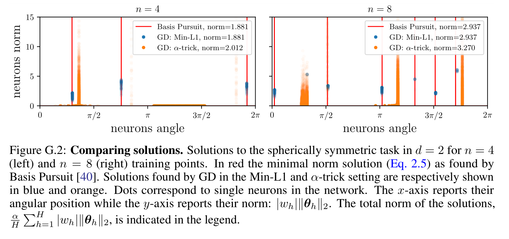
Numerical tests of the theory (ii)
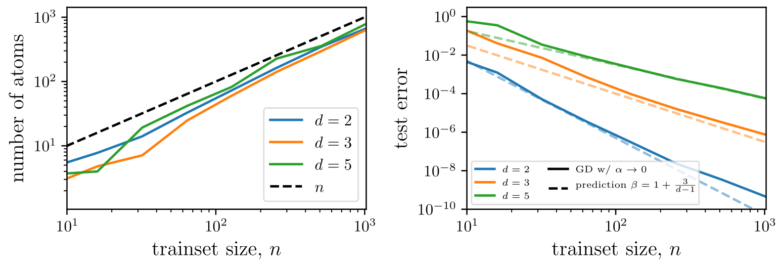

We show here the agreement between theory and
experiments for a smooth target:
- \(\alpha-\)trick:
Predictions:
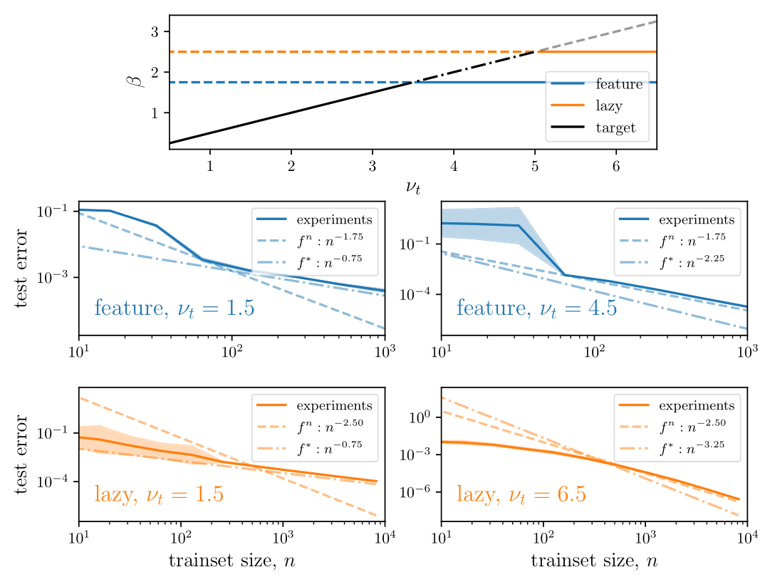
To sum up
For fully-connected networks
-
Feature > Lazy for anisotropic tasks;
- Feature < Lazy if task is constant or smooth along directions that require a continuous distribution of neurons to be represented. In this case the feature predictor becomes sparse and overfits the training set:

e.g.
Bach (2017);
Chizat and Bach (2020); Ghorbani et al. (2019, 2020); Paccolat et al. (2020);
Refinetti et al. (2021);
Yehudai, Shamir (2019)...
Does (2.) hold for FCNs on image datasets?
Evidence for overfitting along diffeomorphisms in image datasets

We argue that the view proposed also holds for images as:
-
Neurons distribution becomes sparse in the feature regime;
- The predictor in the feature regime is less smooth than lazy along directions for which the target should have little variations, i.e. diffeomorphisms.


Conclusions and open questions
-
Central result: learning features can be detrimental if the task varies smoothly along transformations that are not adequately captured by the architecture
(for FCNs: rotations, translations, diffeomorphisms). This result relies on- the sparsity of the feature solution;
- predictions of the gen. error decay when learning GRF on the sphere;
- empirical evidence when learning to classify images.
- Open question: what are the benefits of learning features in modern architectures?