Exploring Explaining Methods in Multi-Label Problems
and Complementary Regularization Strategies
in Weakly Supervised Semantic Segmentation
University of Campinas
Doctoral Qualifying Exam
Candidate: Lucas Oliveira David
Advisor: Prof. Dr. Zanoni Dias
Co-advisor: Prof. Dr. Hélio Pedrini


Schedule
1. Introduction
2. Related Work
3. Research Proposal
4. Preliminary Results
5. Final Considerations
Schedule
1. Introduction
2. Related Work
3. Research Proposal
4. Preliminary Results
5. Final Considerations
Schedule
2. Related Work
3. Research Proposal
4. Preliminary Results
5. Final Considerations
1. Introduction
1.3. Weakly Supervised Semantic Segmentation
1.4. Research Goals
1.2. Explaining and Interpreting Models
1.1. Representation Learning
Figure 1: Samples in the ImageNet 2012 dataset¹. Source: cs.stanford.edu/people/karpathy/cnnembed.
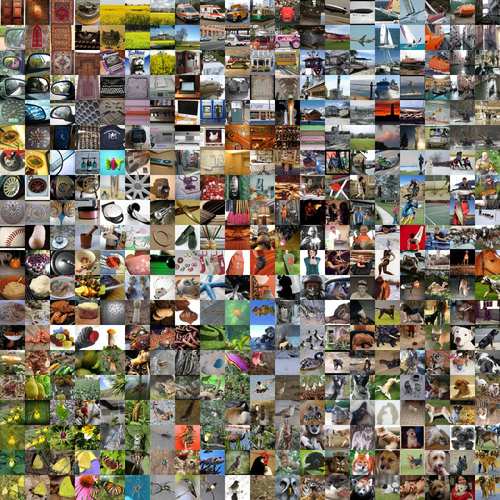
¹ O. Russakovsky, J. Deng, H. Su, J. Krause, S. Satheesh, S. Ma, Z. Huang, A. Karpathy, A. Khosla, M. Bernstein and A.C. Berg. Imagenet Large Scale Visual Recognition Challenge.
In International Journal of Computer Vision, 115, pp.211-252, 2015.
Representation Learning Introduction
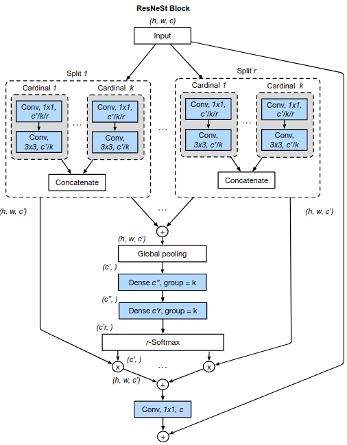
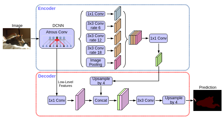
Figure 2: VGG-19, 34Plain and ResNet34 architectures¹.
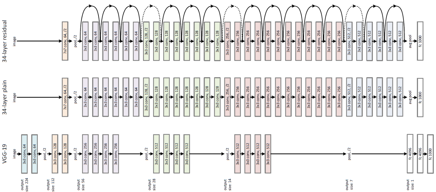
Figure 3: DeepLabV3+ architecture².
Figure 4: Split-Attention Block in the ResNeSt architecture.³
¹ Source: K. He, X. Zhang, S. Ren, and J. Sun. Deep Residual Learning for Image Recognition. In Conference on Computer Vision and Pattern Recognition (CVPR), pp. 770-778. 2016.
² Source: L. Chen, Y. Zhu, G. Papandreou, F. Schroff, and H. Adam. Encoder-decoder with Atrous Separable Convolution for Semantic Image Segmentation. In European Conference on Computer Vision (ECCV), pp. 801-818. 2018.
³ Source: H. Zhang, C. Wu, Z. Zhang, Y. Zhu, H. Lin, Z. Zhang, Y. Sun et al. ResNeSt: Split-Attention Networks. In Conference on Computer Vision and Pattern Recognition (CVPR), pp. 2736-2746. 2022.
Representation Learning Introduction
Complex Architectures Representation Learning
¹ N. Burkart, and M.F. Huber. A survey on the explainability of supervised machine learning. In Journal of Artificial Intelligence Research, 70, pp.245-317., 73, pp.1-15. 2018.
² M. Tan, and Q. Le. EfficientNet: Rethinking model scaling for convolutional neural networks. In International conference on machine learning. PMLR. 2019.
But can we thrust their predictions?
And why do we have to?¹
- Critical operations
- Medical diagnostics
- Finance systems
- Accountability and failure mitigation
Figure 5: Models of various architectures, pre-trained over ImageNet. Source: Tan and Le².
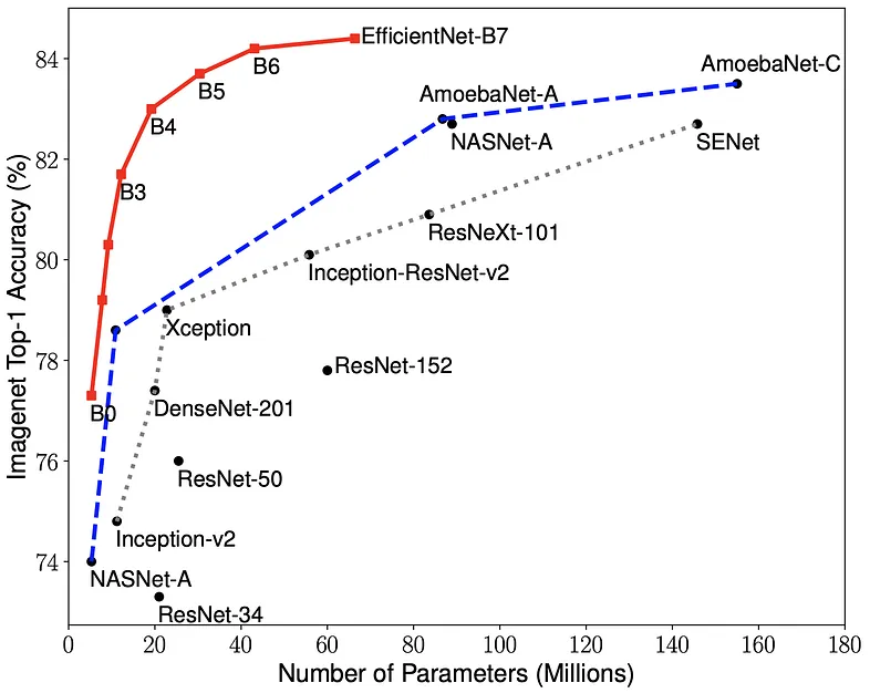
Models with millions of parameters
are now the standard.
Schedule
2. Related Work
3. Research Proposal
4. Preliminary Results
5. Final Considerations
1. Introduction
1.3. Weakly Supervised Semantic Segmentation
1.4. Research Goals
1.2. Explaining and Interpreting Models
1.1. Representation Learning
Explaining and Interpreting Models Introduction
"An explanation is the collection of features of the interpretable domain, that have contributed for a given example to produce a decision (e.g., classification or regression).¹"
¹ G. Montavon, W. Samek, and K.R. Müller. Methods for Interpreting and Understanding Deep Neural Networks. In Digital Signal Processing, 73, pp.1-15. 2018.
² M. D. Zeiler and R. Fergus. Visualizing and understanding convolutional networks. In European Conference on Computer Vision (ECCV), pages 818–833. Springer, 2014.
"An interpretation is the mapping of an abstract concept (e.g., a predicted class) into a domain that the human can make sense of.¹"
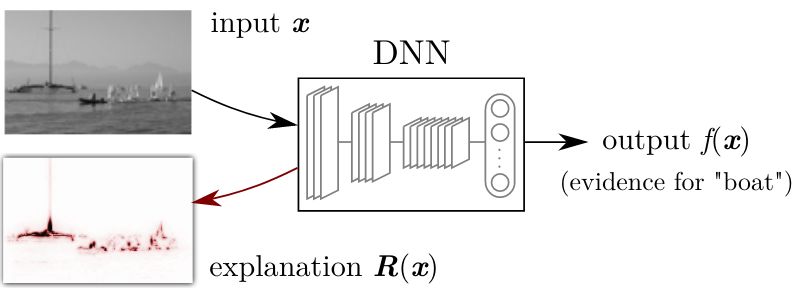
Figure 7: Example of the LRP method being applied to explain the prediction of class boat, given the image x. Source: Montavon et al.¹

Figure 6: Illustration of Activation Maximization² applied to finding the prototypes for each class in the MNIST dataset. Source: Montavon et al.¹
In Computer Vision Explainable AI
Explainability and explainable predictions:
¹ K. Simonyan, A. Vedaldi, A. Zisserman. Deep inside convolutional networks: Visualising image classification models and saliency maps. arXiv preprint arXiv:1312.6034. 2013.
² D. Smilkov, N. Thorat, B. Kim, F. Viégas, M. Wattenberg. SmoothGrad: removing noise by adding noise. arXiv preprint arXiv:1706.03825. 2017.
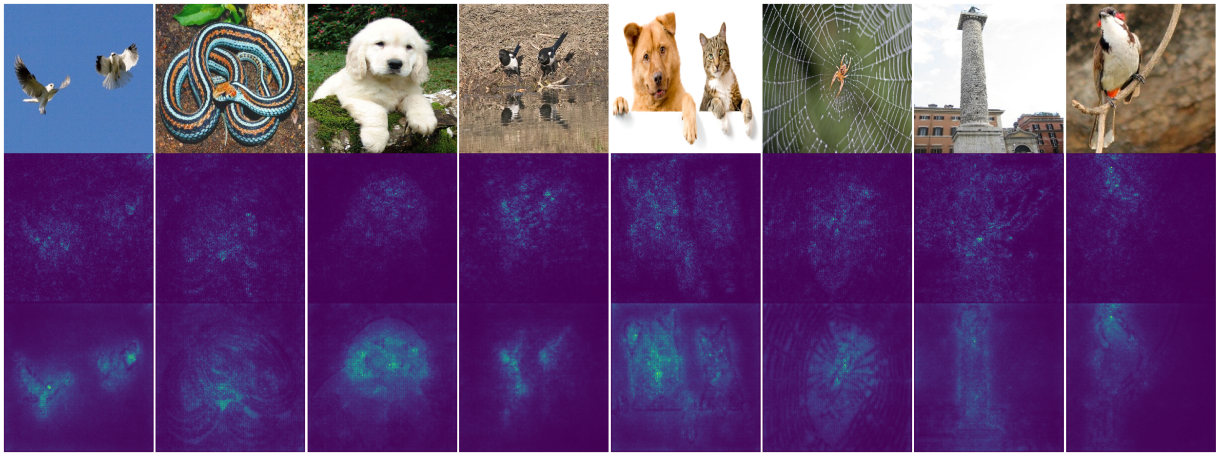
Figure 8: Sensitivity maps produced by Vanilla Gradient¹ (second row) and Smooth-Grad² (third row), when employed to explain the predictions made by a Xception model. Source: keras-explainable/methods/saliency/smoothgrad.
Interesting Properties:
- Completeness
- Weak dependence
- Class-specificity
In Computer Vision Explainable AI
Leveraging internalized knowledge
to solve different tasks:

Figure 9: Sensitivity maps produced by Smooth-Grad.
Source: keras-explainable/methods/saliency/smoothgrad.
Schedule
2. Related Work
3. Research Proposal
4. Preliminary Results
5. Final Considerations
1. Introduction
1.3. Weakly Supervised Semantic Segmentation
1.4. Research Goals
1.2. Explaining and Interpreting Models
1.1. Representation Learning
Semantic (and others) Segmentation Introduction
¹ H. Xiao, D. Li, H. Xu, S. Fu, D. Yan, K. Song, and C. Peng. Semi-Supervised Semantic Segmentation with Cross Teacher Training. Neurocomputing, 508, pp.36-46. 2022.
² H. Zhao, X. Qi, X. Shen, J. Shi, and J. Jia. ICNet for Real-Time Semantic Segmentation on High-Resolution Images. In European Conference on Computer Vision (ECCV), pp. 405-420. 2018.
³ L. Chan, M.S. Hosseini. and K.N. Plataniotis. A Comprehensive Analysis of Weakly-Supervised Semantic Segmentation in Different Image Domains. In International Journal of Computer Vision, 129, pp.361-384. 2021.
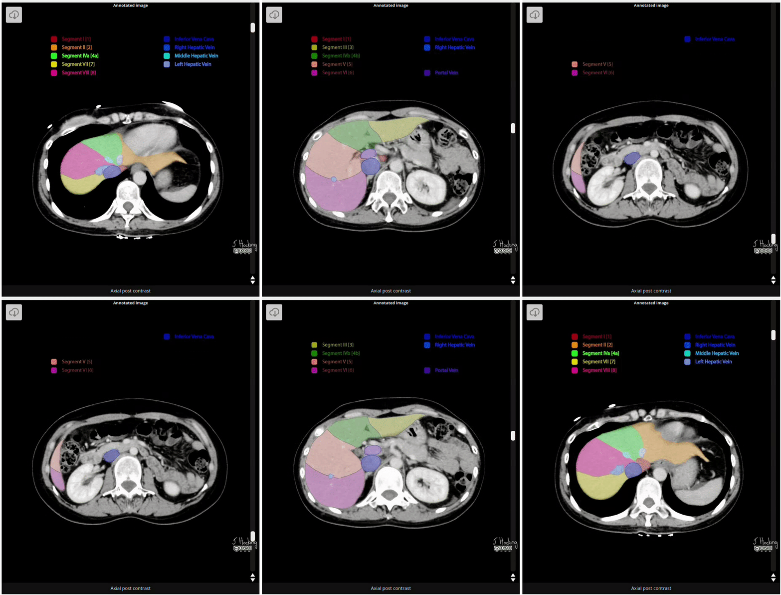
Figure 15: Example of annotated CT Scan image. Source: https://radiopaedia.org/cases/liver-segments-annotated-ct-1
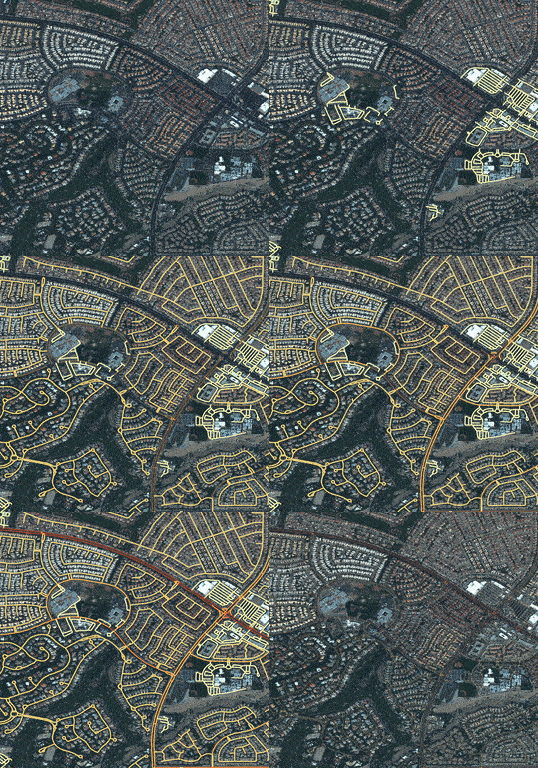
Figure 13: Example of road segmentation in SpaceNet dataset. Source: https://www.v7labs.com/open-datasets/spacenet


Figure 14: Example of (a) morphological and (b) functional segmentation of samples in the Atlas of Digital Pathology dataset. Source: L. Chan et al.
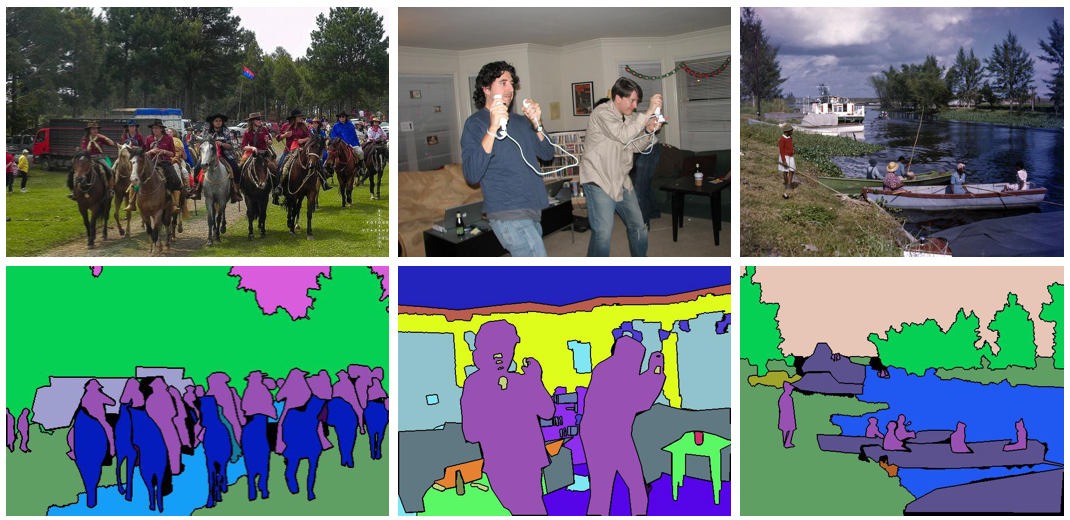
Figure 11: Example of samples and ground-truth panoptic segmentation annotation from the MS COCO 2017 dataset. Source: https://cocodataset.org/#panoptic-2020.
Figure 12: Example of semantic segmentation produced by ICNet for a video sample in the Cityscapes dataset. Source: https://gitplanet.com/project/fast-semantic-segmentation.
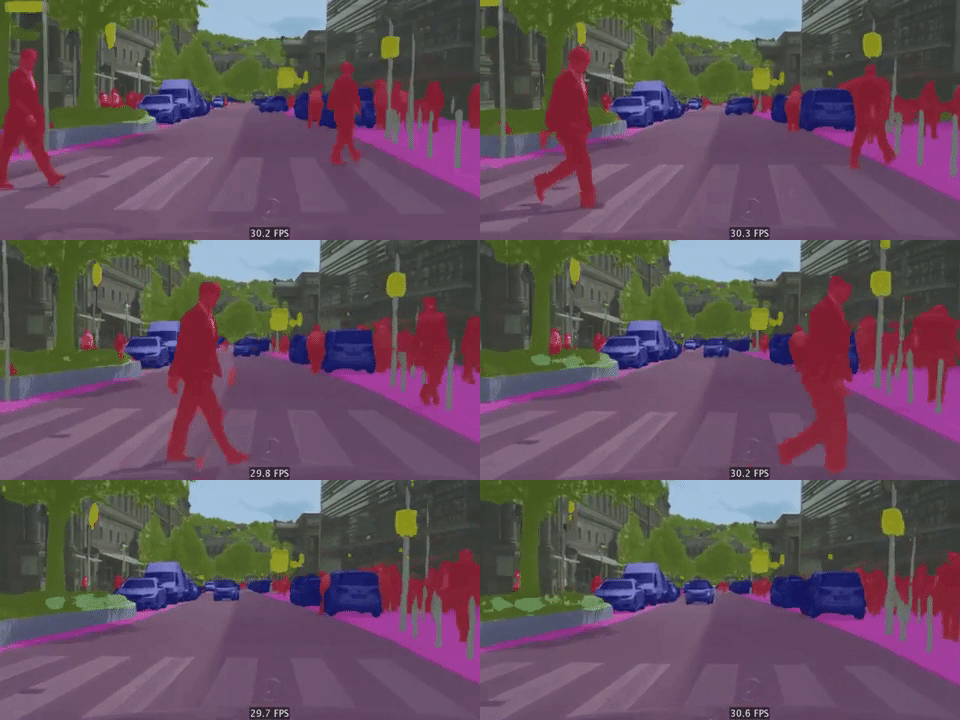
Figure 10: Samples, proposals¹ and ground-truth segmentation annotation from the Pascal VOC 2012 dataset.
How It is Done? Semantic Segmentation
¹ J. Long, E. Shelhamer, and T. Darrell. Fully Convolutional Networks for Semantic Segmentation. In IEEE Conference on Computer Vision and Pattern Recognition (CVPR), pp. 3431-3440. 2015.
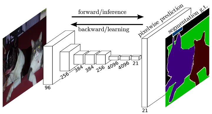
Figure 16: Fully Convolutional Network (FCN) architecture¹, mapping image samples to their respective semantic segmentation maps.
This information needs the be known and available at training time.
Equation 1: The (naive) categorical cross-entropy loss function.
Figure 18: Segmentation annotation example using Dataloop. Source: https://dataloop.ai/docs.
Figure 17: Segmentation annotation example using RoboFlow. Source: https://blog.roboflow.com/semantic-segmentation-roboflow.
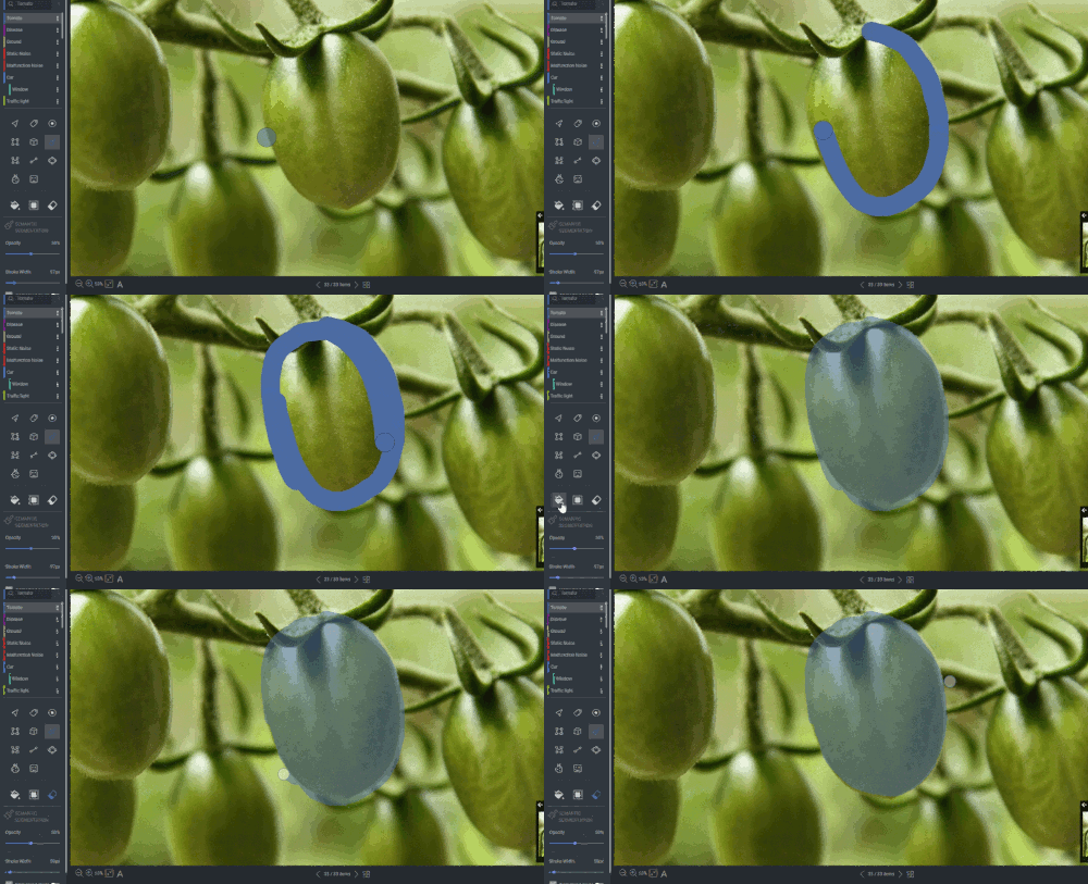
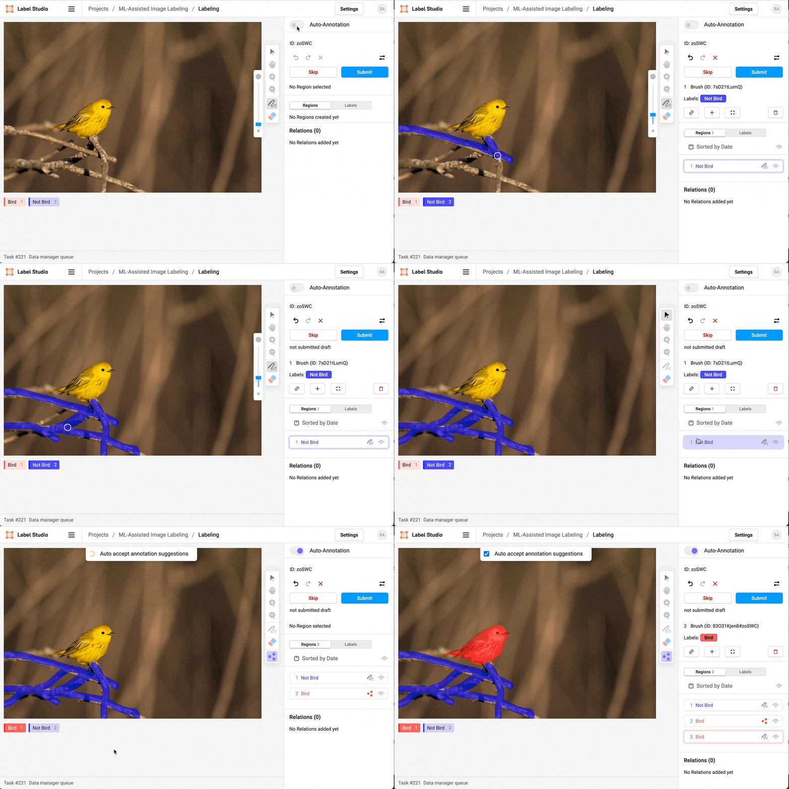
Figure 19: Segmentation annotation example using LabelStudio. Source: https://labelstud.io/blog/perform-interactive-ml-assisted-labeling-with-label-studio-1-3-0.
(Fully) Supervised Learning Semantic Segmentation
Coarse annotations are quickly drawn, but lack quality (e.g., precision);
Detailed annotations take time, patience, people and resources;
Assisting labeling tools can speed up this task.
(Weakly) Supervised Learning Semantic Segmentation
¹ O. Russakovsky, J. Deng, H. Su, J. Krause, S. Satheesh, S. Ma, Z. Huang, A. Karpathy, A. Khosla, M. Bernstein and A.C. Berg. Imagenet Large Scale Visual Recognition Challenge.
In International Journal of Computer Vision, 115, pp.211-252, 2015.
Figure 20: Samples in the ImageNet 2012 dataset¹. Source: cs.stanford.edu/people/karpathy/cnnembed.

Schedule
2. Related Work
3. Research Proposal
4. Preliminary Results
5. Final Considerations
1. Introduction
1.3. Weakly Supervised Semantic Segmentation
1.4. Research Goals
1.2. Explaining and Interpreting Models
1.1. Representation Learning
Research Goals Introduction
-
To study Class-Specific XAI methods in the multi-label scenarios
-
To study promising weakly supervised strategies and to propose new ones
-
To investigate the behavior of WSSS solutions to more complex boundary cases, such as long-tail and ambiguous functional segmentation problems
Schedule
1. Introduction
2. Related Work
3. Research Proposal
4. Preliminary Results
5. Final Considerations
Schedule
1. Introduction
2. Related Work
3. Research Proposal
4. Preliminary Results
5. Final Considerations
2.1. (Visual) Explainable Artificial Intelligence (XAI)
2.2. Weakly Supervised Semantic Segmentation (WSSS)
Explainable AI Related Work
Equation 2: Saliency map for the concept c of a model S with respect to an input image x, generated by the (Vanilla) Gradients method¹.
¹ K. Simonyan, A. Vedaldi, A. Zisserman. Deep inside convolutional networks: Visualising image classification models and saliency maps. arXiv preprint arXiv:1312.6034. 2013.
² S. Srinivas and F. Fleuret. Full-gradient representation for neural network visualization. In Advances in neural information processing systems, 32. 2019.
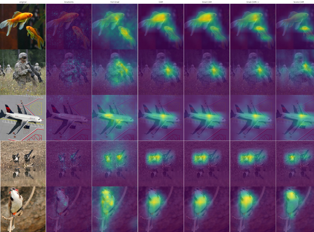
Figure 21: Sensitivity maps produced by Vanilla Gradient¹ (2nd col) and Full-Grad² (3rd col), when employed to explain the predictions made by a ResNet50 model.
Source: keras-explainable.
Equation 3: Saliency map for the concept c of a model S with respect to an input image x, generated by the Full-Gradient method².
Lack class-sensibility
Expensive to compute
Class Activation Mapping Explainable AI
¹ B. Zhou, A. Khosla, A. Lapedriza, A. Oliva, and A. Torralba. Learning Deep Features for Discriminative Localization. In Conference on Computer Vision and Pattern Recognition (CVPR), pp. 2921-2929. 2016.
Equation 4: Feed-Forward for a for Convolutional Networks containing GAP layers and the formulation for CAM¹.
Class Activation Mapping Explainable AI
¹ B. Zhou, A. Khosla, A. Lapedriza, A. Oliva, and A. Torralba. Learning Deep Features for Discriminative Localization. In Conference on Computer Vision and Pattern Recognition (CVPR), pp. 2921-2929. 2016.
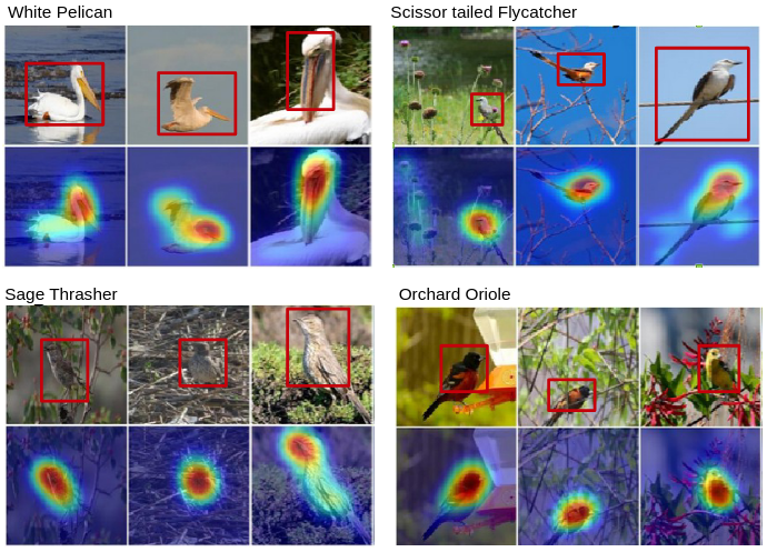
Figure 22: Examples of CAMs and approximate bounding boxes found for different birds in the CUB200 dataset. Source: Zhou et al.¹
Extensions and Alternatives CAM-Based Explaining Methods
¹ R. R. Selvaraju, M. Cogswell, A. Das, R. Vedantam, D. Parikh, and D. Batra. Grad-CAM: Visual Explanations from Deep Networks via Gradient-Based Localization. In International Conference on Computer Vision, pp. 618-626. 2017.
Equation 5: Definition for Grad-CAM visual explaining method, for an arbitrary convolutional network f.
Grad-CAM
Goal: to explain more complex networks, with non-linear (and yet smooth) operations after the GAP layer.
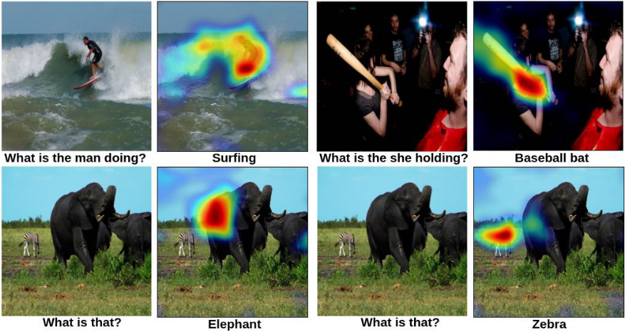
Figure 23: Examples of Grad-CAM being utilized to explaing a Visual Questioning Network based on convolutional layers and LSTM layers. Source: Selvaraju et al.¹
¹ A. Chattopadhay, A. Sarkar, P. Howlader, and V. N. Balasubramanian. Grad-CAM++: Generalized gradient-based visual explanations for deep convolutional networks.
In Winter Conference on Applications of Computer Vision (WACV), pp. 839-847. IEEE, 2018.
Equation 6: Definition of Grad-CAM++ visual explaining method.
Grad-CAM++
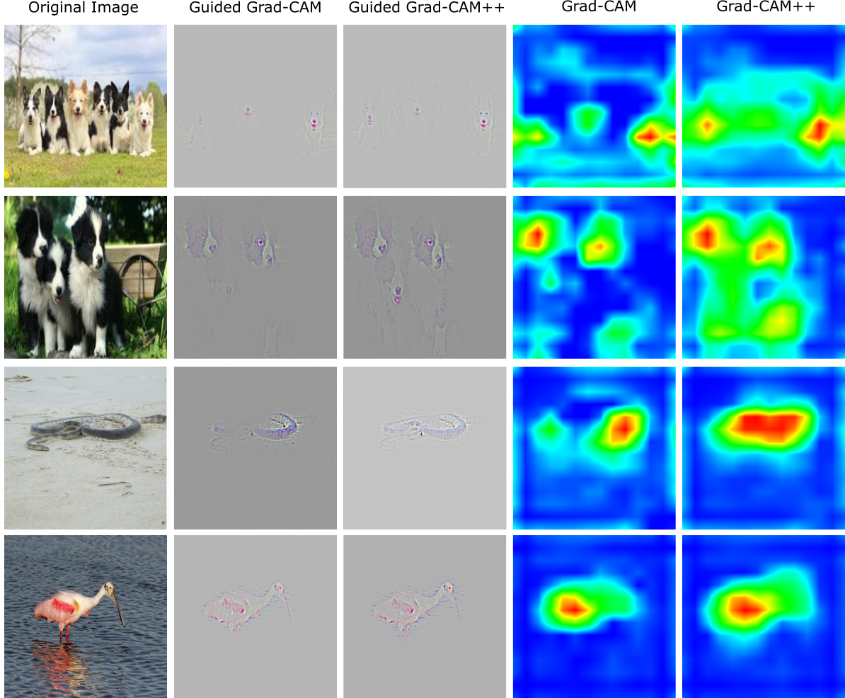
Goal: to activate homogeneously over all instances of the explained concept lying the the visual receptive field.
Extensions and Alternatives CAM-Based Explaining Methods
Figure 24: Grad-CAM and Grad-CAM++ being applied to samples in the ImageNet dataset. Source: Chatopadhay et al.¹
¹ H. Wang, Z. Wang, M. Du, F. Yang, Z. Zhang, S. Ding, P. Mardziel, and X. Hu. Score-CAM: Score-weighted visual explanations for convolutional neural networks. In Conference on Computer Vision and Pattern Recognition Workshops (CVPR), pp. 24-25. 2020.
Equation 7: Definition of the Score-CAM visual explaining method¹.
Score-CAM
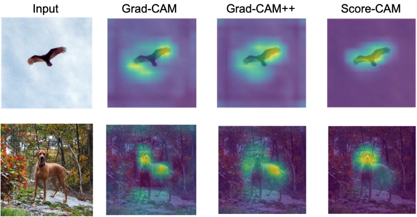
Goal: to combine the many activation maps, weighted by their contribution towards the Average Drop % metric.
Extensions and Alternatives CAM-Based Explaining Methods
Figure 25: Examples of sensitivity maps obtained from Grad-CAM, Grad-CAM++ and Score-CAM.
Source: Wang et al.¹
Schedule
1. Introduction
2. Related Work
3. Research Proposal
4. Preliminary Results
5. Final Considerations
2.1. (Visual) Explainable Artificial Intelligence
2.2. Weakly Supervised Semantic Segmentation (WSSS)
Weakly Supervised Semantic Segmentation Related Work
Coarse Semantic Segmentation Priors WSSS
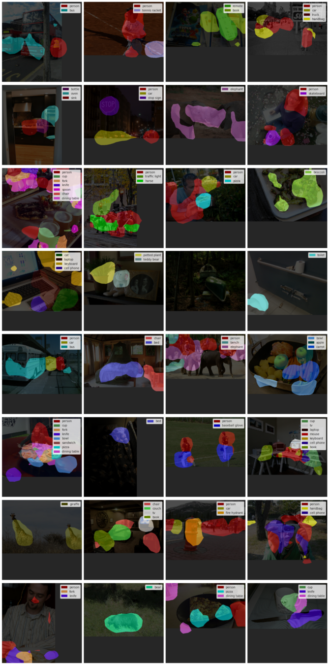
Figure 26: Semantic Segmentation Priors produced by thresholding CAMs devised from a ResNet101 model trained over MS COCO 2017 dataset.

Refinement of Segmentation Masks WSSS
- Architectural
- Pixel neighborhood affinity and similarity
- Many other strategies: Seed-Expand-Constrain; region semantic-based clustering; token-based similarity matching, etc.
Refinement of Segmentation Masks WSSS
¹ Z. Wu, C. Shen, and A. Van Den Hengel. Wider or deeper: Revisiting the resnet model for visual recognition. In Pattern Recognition, 90, pp.119-133. 2019.
- Architectural
(2048, 16, 16)
(3, 512, 512)
(4096, 64, 64)
(3, 512, 512)
- Fewer layers, more units
- "Bottleneck" blocks
- Strong dropout
- Dilation
FC Conditional Random Fields Refinement of Segmentation Masks
¹ P. Krähenbühl, and V. Koltun. Efficient inference in fully connected CRFs with gaussian edge potentials. In Advances in Neural Information Processing Systems, 24. 2011.
pairwise
unary
smoothness kernel
label compatibility function (learnable)
appearance kernel
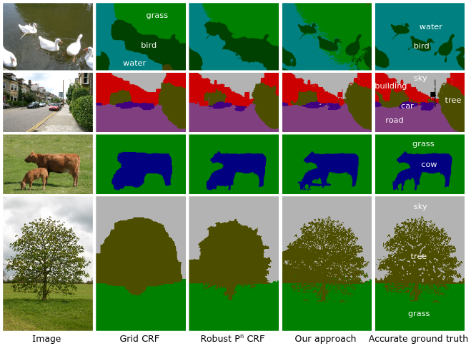
Figure 27: Qualitative results of dCRF. Source: Krähenbühl and Koltun¹.

Pixel Semantic Affinity Refinement of Segmentation Masks
¹ J. Ahn, and S. Kwak. Learning pixel-level semantic affinity with image-level supervision for weakly supervised semantic segmentation. In Conference on Computer Vision and Pattern Recognition (CVPR), pp. 4981-4990. 2018.
Inference
Training
Pairs extraction
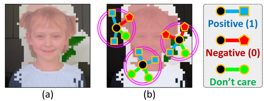
Figure 5: Illustration of pairs of pixels selected for affinity evaluation. Source: Ahn and Kwak¹.
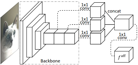
Figure 5: AffinityNet architecture. Source: Ahn and Kwak¹.
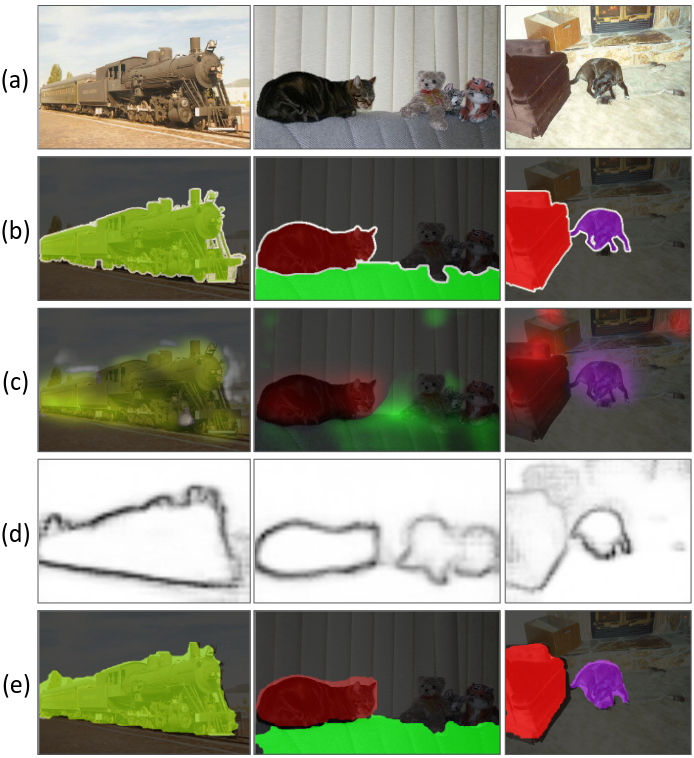
Figure 28: Qualitative results of random walk using Affinity Network. Source: Ahn and Kwak¹.
Puzzle-CAM Better Segmentation Priors
¹ S. Jo, and I. Yu. Puzzle-CAM: Improved localization via matching partial and full features. In IEEE International Conference on Image Processing (ICIP), pp. 639-643. IEEE, 2021.

Figure 29: Puzzle-CAM architecture: the input image is forwarded into the model, producing the global stream. Concomitantly, the input is also cut into four "puzzle" pieces and forward separately, which compose the "local" stream when merged. Source: Jo and Yu¹.
¹ H. Kweon, S. H. Yoon, H. Kim, D. Park, and K. J. Yoon. Unlocking the potential of ordinary classifier: Class-specific adversarial erasing framework for weakly supervised semantic segmentation. In IEEE/CVF International Conference on Computer Vision (ICCV), pp. 6994-7003. 2021.
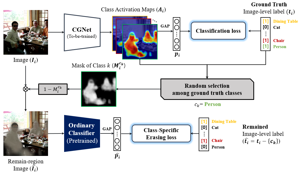
Figure 30: OC-CSE architecture: the input image is forwarded into the CGNet, producing a mask for a random class k. The mask is then used to erase objects of k in the image and fed to a OC (fixed) model. Weights are adjusted so the mask provides a comprehensive erasure of the objects. Source: Jo and Yu¹.
OC-CSE Better Segmentation Priors
C²AM Better Segmentation Priors


Training
Inference
Refined
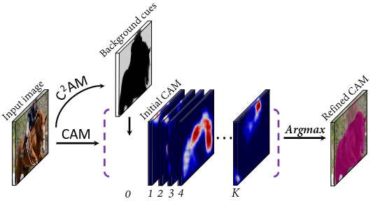
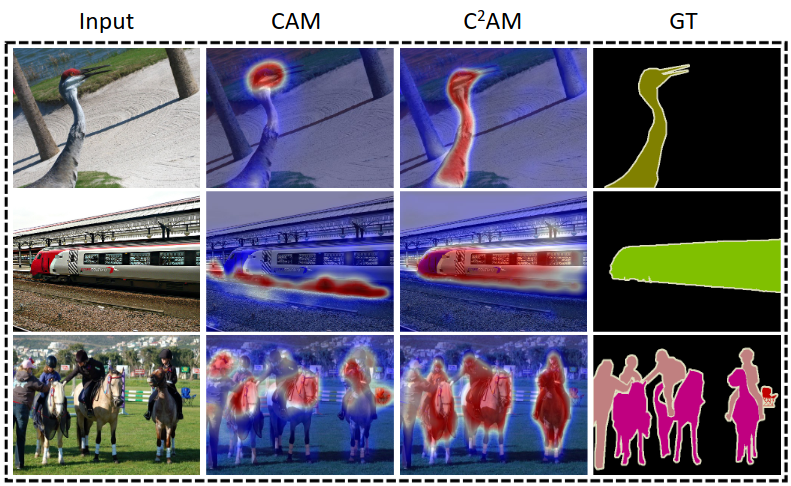
Figure 31: C²AM processing pipeline. Source: Xie et al.¹
¹ J. Xie, J. Xiang, J. Chen, X. Hou, X. Zhao, and L. Shen. Contrastive learning of class-agnostic activation map for weakly supervised object localization and semantic segmentation. arXiv preprint arXiv:2203.13505. 2022.
Schedule
1. Introduction
2. Related Work
3. Research Proposal
4. Preliminary Results
5. Final Considerations
Schedule
1. Introduction
2. Related Work
3. Research Proposal
4. Preliminary Results
5. Final Considerations
3.2. Proposed Approach and Research Questions
3.3. Experimental Setup
3.1. Motivation
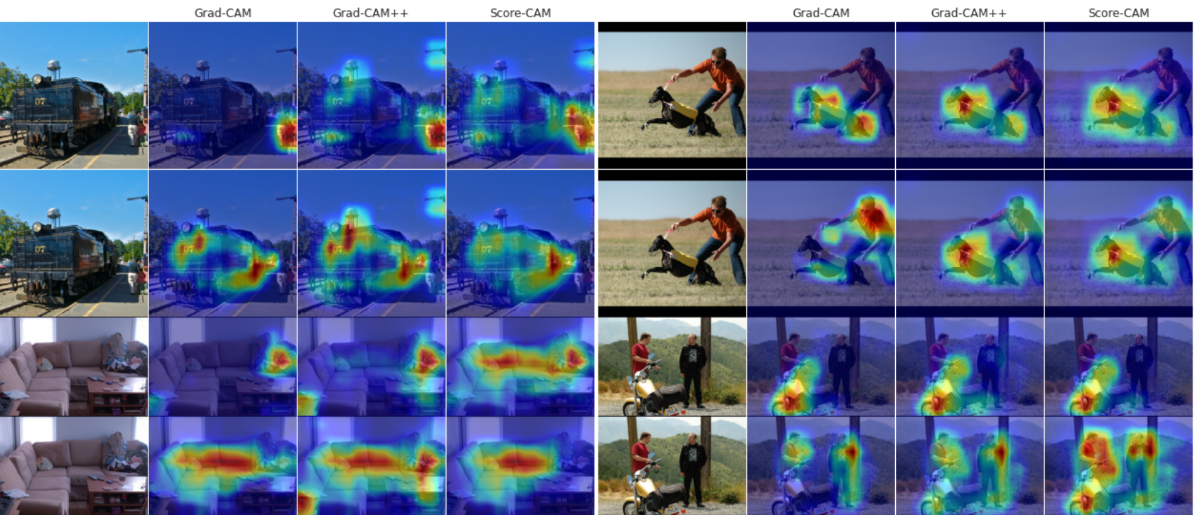
Figure 32: Examples of sensitivity maps obtained from Grad-CAM, Grad-CAM++ and Score-CAM over samples in the Pascal VOC 2007 dataset. Predictions being explained are: person, train, person, sofa, dog, person, motorcycle, and person. Source: David et al.¹
¹ L. David., H. Pedrini., and Z. Dias. MinMax-CAM: Improving focus of CAM-based visualization techniques in multi-label problems. In 17th International Joint Conference on Computer Vision, Imaging and Computer Graphics Theory and Applications - Volume 4: VISAPP, pages 106–117. INSTICC, SciTePress, 2022.
Motivation Research Proposal
Motivation Research Proposal
¹ W. Sun, J. Zhang, Z. Liu, Y. Zhong, N. Barnes. GETAM: Gradient-weighted element-wise transformer attention map for weakly-supervised semantic segmentation. arXiv preprint arXiv:2112.02841. 2021 Dec 6.
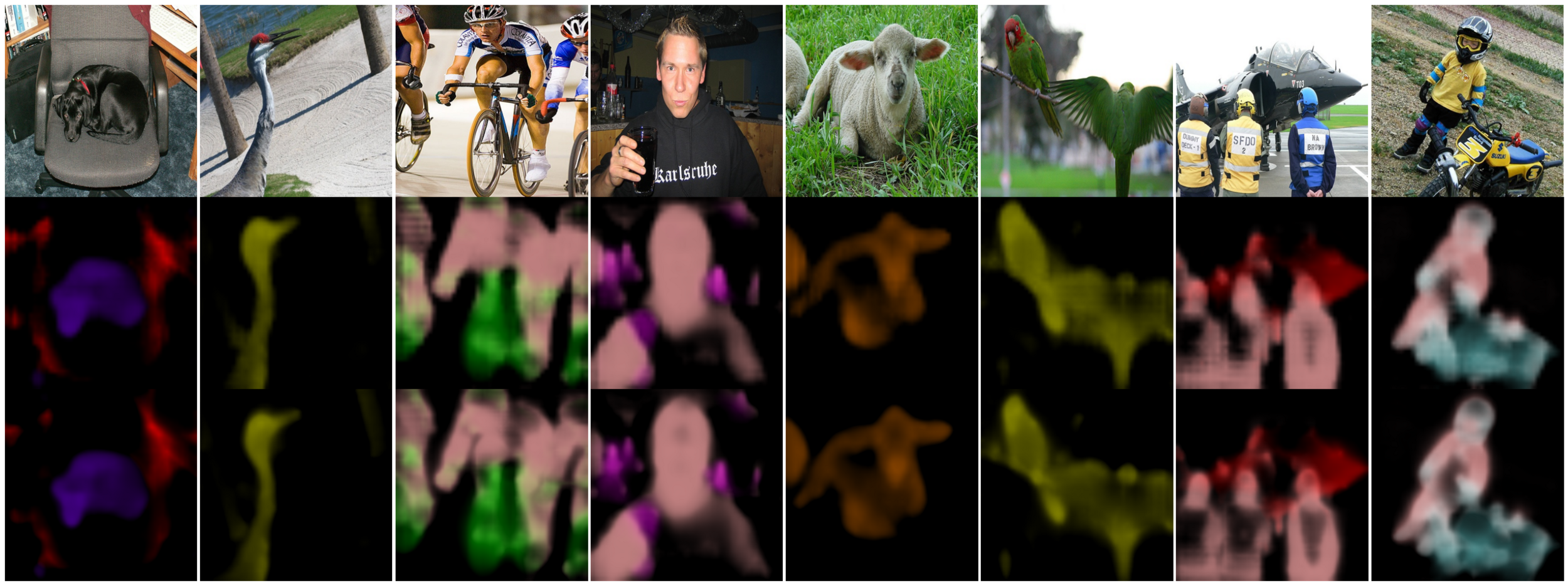
Figure 33: Semantic Segmentation priors produced by a ResNet38d model trained with OC-CSE. CAMs were generated using Grad-CAM and Test-Time Augmentation (TTA). Source: keras-explainable/wsol.

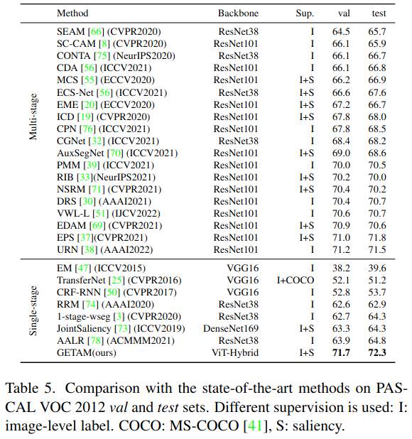
Figure 34: mIoU measured over Pascal VOC 2012 testing dataset. Source: https://paperswithcode.com/sota/semantic-segmentation-on-pascal-voc-2012.
Source: Sun et al.¹
Schedule
1. Introduction
2. Related Work
3. Research Proposal
4. Preliminary Results
5. Final Considerations
3.2. Proposed Approach and Research Questions
3.3. Experimental Setup
3.1. Motivation
- How do Explainable AI methods behave in multi-label scenarios?
- Can cross-contributions be erased from the CAMs produced by Grad-CAM?
1. Exploration of Explainable AI Methods in Multi-Label Problems
Proposed Approach Research Proposal
- Can complementary strategies be conjointly employed to improve WSSS?
- Is adversarial CAM generation beneficial to WSSS solutions?
- Can context-decoupling help WSSS methods to segment cluttered scenes?
2. Complementary Regularization Strategies in WSSS
Proposed Approach Research Proposal
- Can Visual Transformers improve fine-grain WSSS?
- Can WSSS methods be adapted to Vision Transformers?
3. Exploration of Transformers and Spatial Attention for Highly-Detailed
Segmentation
Proposed Approach Research Proposal
- Can long-tail learning improve WSSS in boundary cases?
- Which features can be drawn from functional segmentation problems to replace visual similarity, a fundamental aspect of WSSS methods?
4. Weak Supervision in Boundary and Difficult Scenarios: Class Unbalance, Long-tail and Functional Segmentation
Proposed Approach Research Proposal
- Can WSSS ensembles improve noisy segmentation priors?
- Is contextual information useful when combining predictions?
- Which tasks share mutual information with Semantic Segmentation?
- Saliency Detection
- Edge Detection
- Instance Segmentation
5. Ensemble of Weakly Supervised Semantic Segmentation Systems
Proposed Approach Research Proposal
Work Schedule Research Proposal
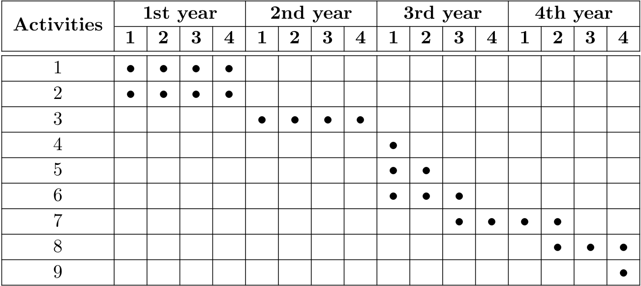
Class attendance and completion of required credits
Exploration of XAI methods in multi-label scenarios
Adversarial and complementary strategies in WSSS
Doctoral Qualifying Exam (EQE)
Participation in "Programa de Estágio Docente" (PED)
Exploration of Transformers and Spatial Attention
Boundary and difficult scenarios
Ensemble of solutions for WSSS
Writing and presentation of Doctoral thesis
Activities
Schedule
1. Introduction
2. Related Work
3. Research Proposal
4. Preliminary Results
5. Final Considerations
3.2. Proposed Approach and Research Questions
3.3. Experimental Setup
3.1. Motivation
Experimental Setup Research Proposal
Environment
Tools
-
Tensorflow and PyTorch
SDumont Supercomputer:
- 4x NVIDIA Volta V100 (training)
- 2x NVIDIA K40 (inference)
Google Colab
- NVIDIA Tesla K80
- mean Intersection over Union (mIoU)
- Pixel Accuracy
- F1 Score
XAI
WSSS
- Increase in Confidence
- Average Drop %
- Average Drop of Others %
- Average Retention %
- Average Retention of Others %
Experimental Setup Research Proposal
Proposed by us.
Metrics
Schedule
1. Introduction
2. Related Work
3. Research Proposal
4. Preliminary Results
5. Final Considerations
Schedule
1. Introduction
2. Related Work
3. Research Proposal
4. Preliminary Results
5. Final Considerations
4.1. Contributions for Explainable AI
4.2. Contributions for WSSS
Contribution towards the classification of class c.
ReLU and GAP omitted for conciseness
Regions that contribute t.t.c. of c, and do not contribute t.t.c. of the adjacent classes.
MinMax-CAM Contributions for Explainable AI
MinMax-CAM Contributions for Explainable AI
Positive contributions t.t.c. of c
Positive contributions t.t.c. of n
Negative contributions t.t.c. of all.
Qualitative Results over VOC MinMax-CAM
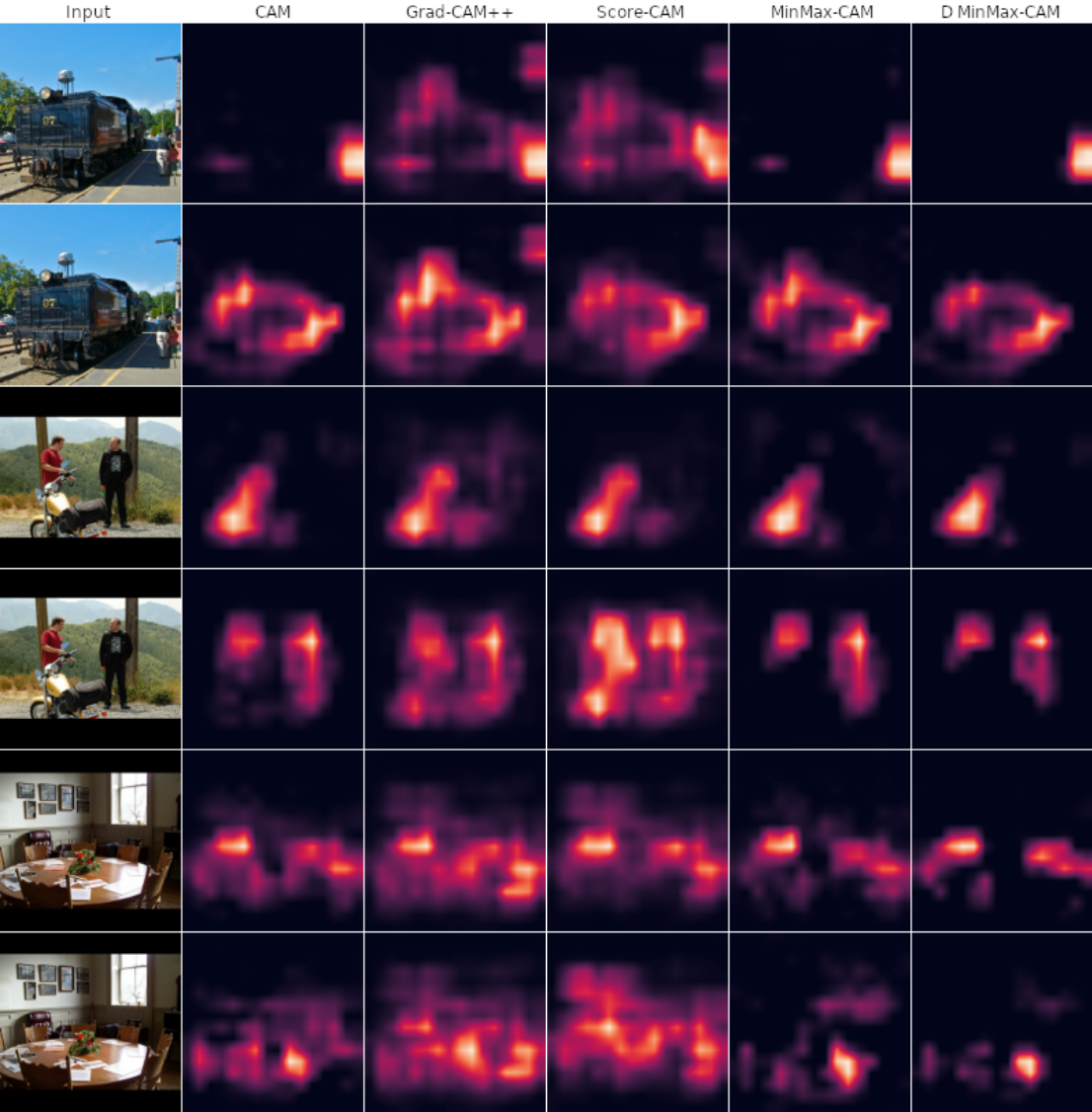
Figure 35: Comparison of CAMs obtained from various XAI methods. Predictions being explained are: person, train, motorcycle, person, chair, and table. Source: David et al.¹
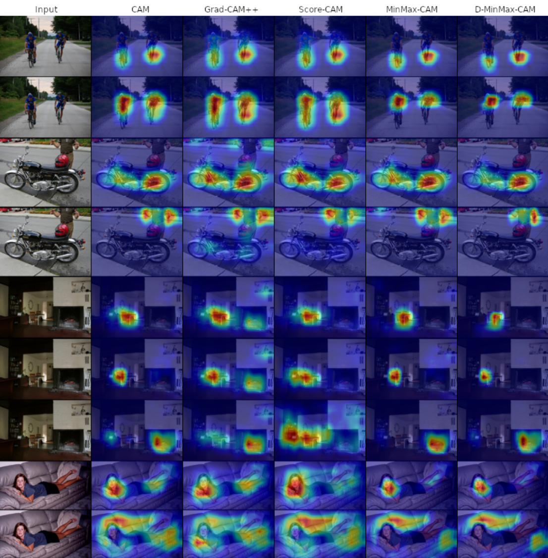
Figure 36: Comparison of sensitivity maps from various XAI methods. Source: David et al.¹

Qualitative Results over COCO 2017 MinMax-CAM
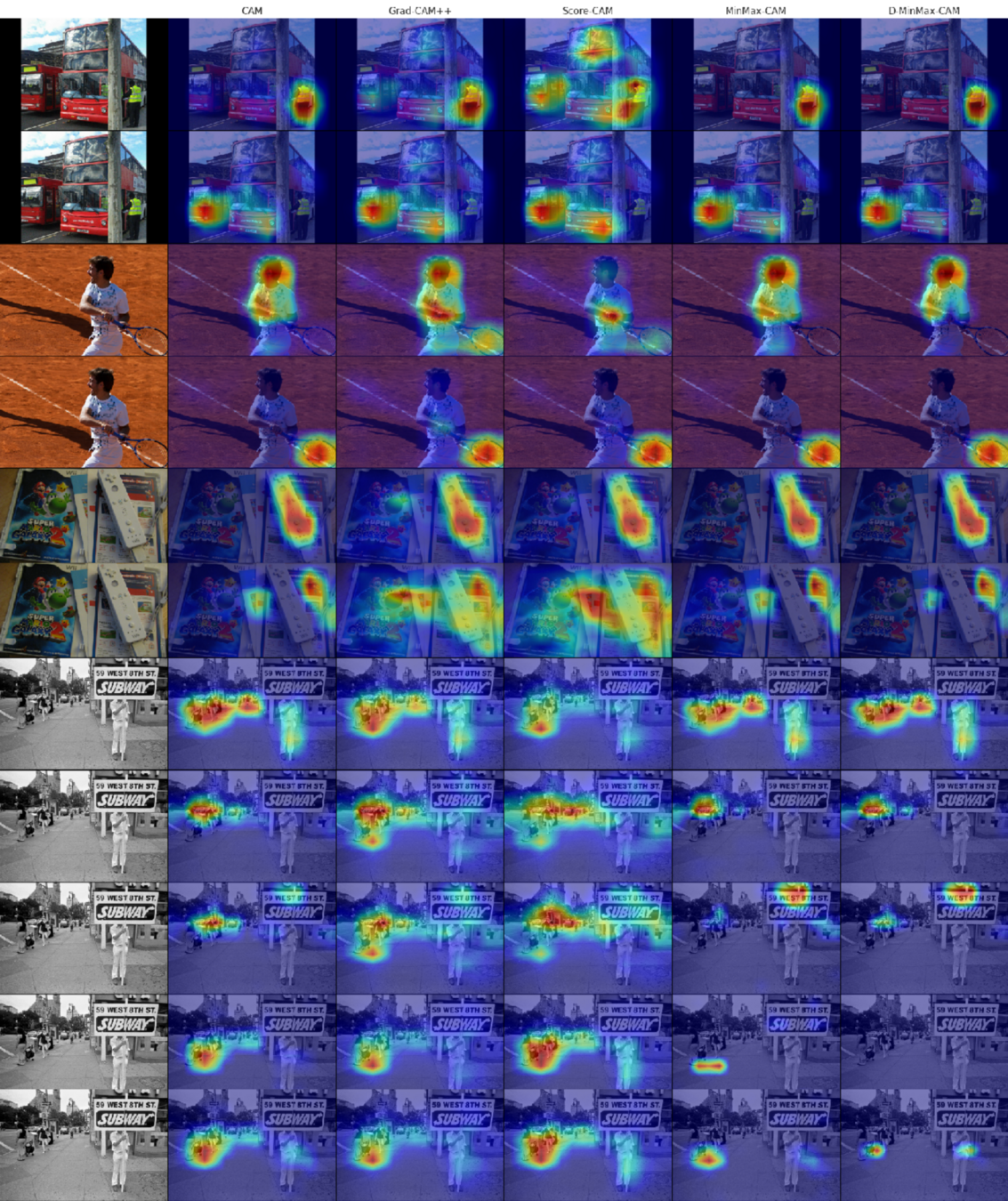
Figure 37: Comparison of sensitivity maps obtained from various XAI methods over the MS COCO 2017 dataset. Source: David et al.¹
Qualitative Results over HPA MinMax-CAM
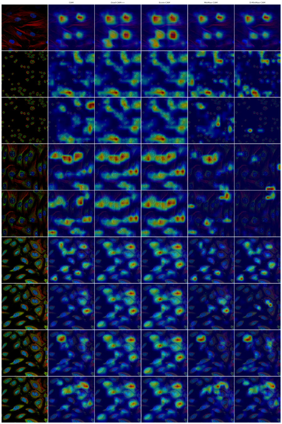
Figure 38: Comparison of sensitivity maps obtained from various XAI methods over the Human Protein Atlas Image Classification dataset. Source: David et al.¹

Quantitative Results MinMax-CAM
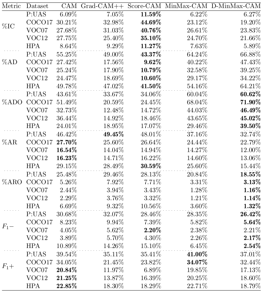
Table 2: Report of metric scores over multiple datasets.
Kernel Usage Regularization Contributions for Explainable AI
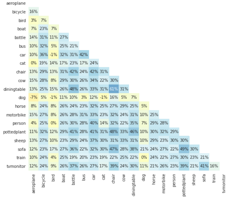
Figure 39: Correlation between different weight vectors in a vanilla (unregularized) sigmoid FC layer. Source: David et al.¹
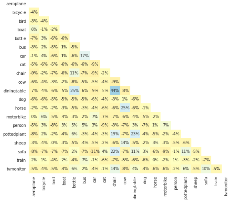
Figure 40: Correlation between different weight vectors in a sigmoid FC layer trained with Kernel Usage Regularization. Source: David et al.¹
Kernel Usage Regularization Contributions for Explainable AI
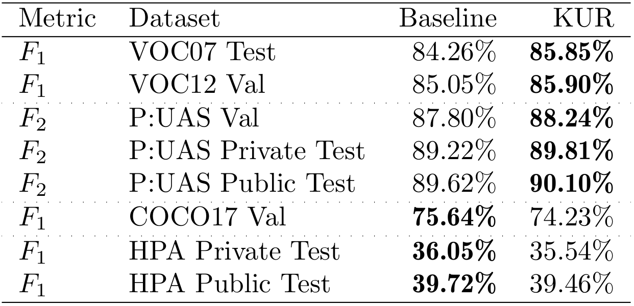
Table 3: Report of classification scores over multiple datasets, considering a baseline classifier the model trained with Kernel Usage Regularization (KUR).
Schedule
1. Introduction
2. Related Work
3. Research Proposal
4. Preliminary Results
5. Final Considerations
4.1. Contributions for Explainable AI
4.2. Contributions for WSSS
Exploration of Complementary WSSS Strategies Contributions for WSSS
Exploration of Complementary WSSS Strategies Contributions for WSSS
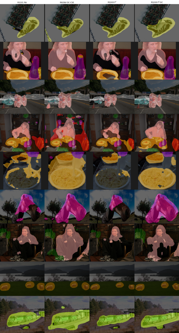
Figure 41: Priors obtained by (from left to right): Vanilla (RandAugment), OC-CSE, Puzzle, P-OC.

Vanilla
OC-CSE
Puzzle
P-OC
Vanilla
OC-CSE
Puzzle
P-OC
P-NOC Contributions for WSSS
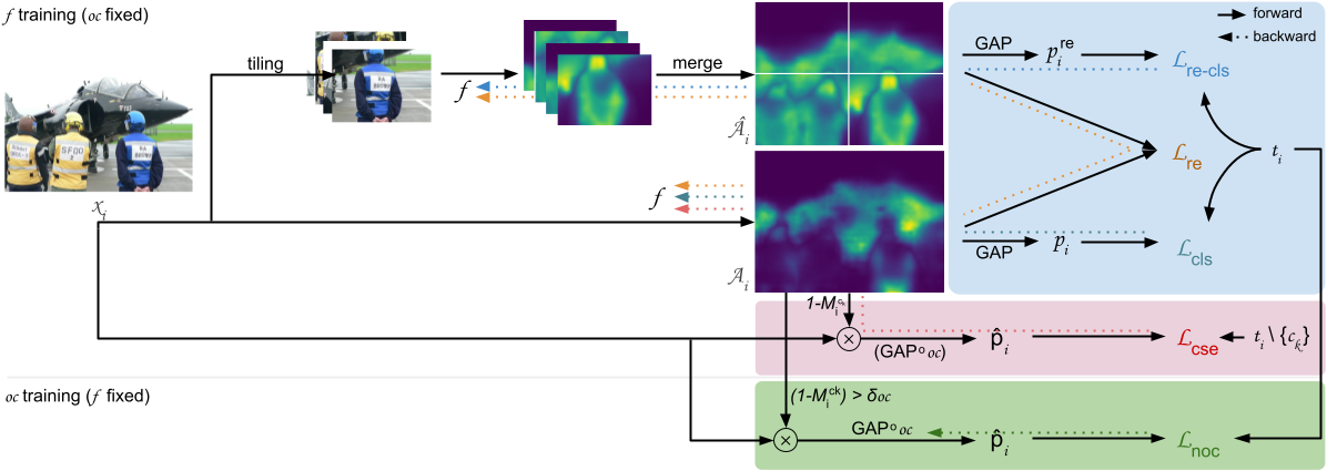
Figure 42: Overview of our adversarial training setup, in which f is optimized considering both Puzzle module and the ordinary classifier oc. f is sub-sequentially fixed and oc is updated to shift its attention towards regions currently ignored by f.
P-NOC Contributions for WSSS
P-NOC Contributions for WSSS
C²AM-H Contributions for WSSS


Figure 43: CAMs produced by a network trained with P-OC, when presented with samples from the Pascal VOC 2012 train set.
Figure 44: Hints obtained by binarizing the CAMs, using a threshold of 0.4.
C²AM-H Contributions for WSSS
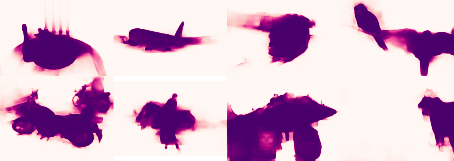
Figure 45: Saliency proposals obtained from a PoolNet model, after being trained with C²AM-H pseudo saliency maps.
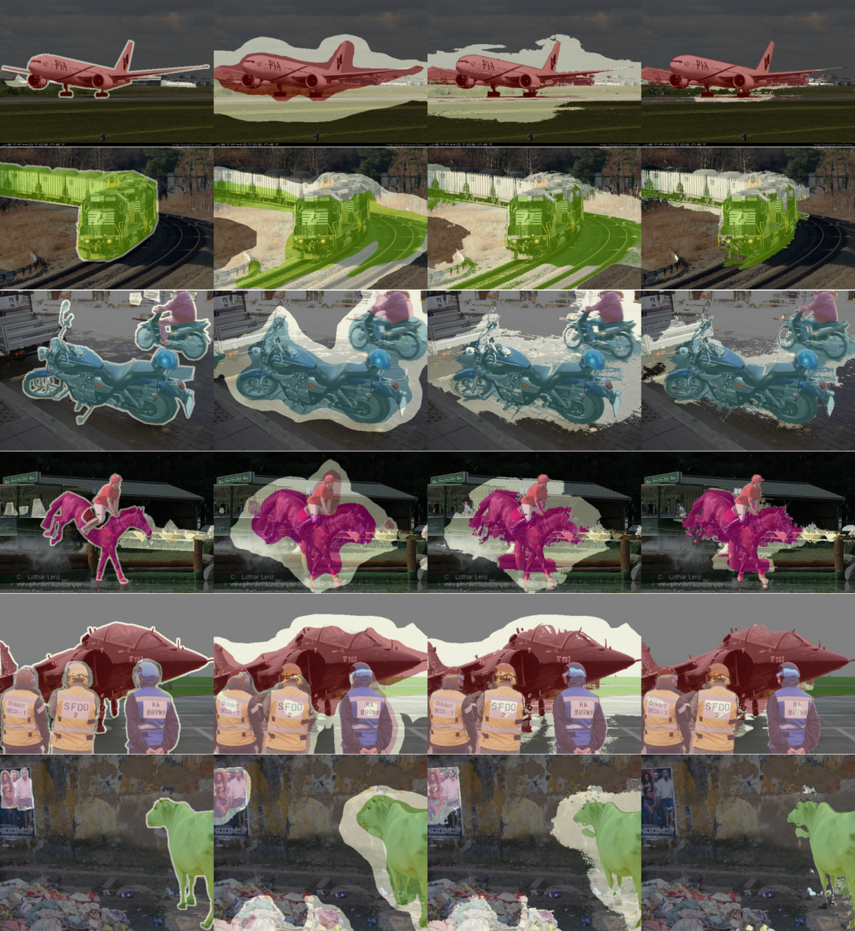
Figure 46: Affinity labels. From left to right: (a) ground-truth maps, (b) coarse priors, (c) priors +dCRF, and (d) priors +C²AM-H +dCRF.
Ablation Studies Contributions for WSSS
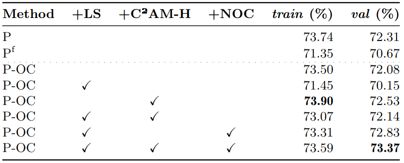
Table 4: Ablation studies of pseudo segmentation masks, measured in mIoU (%) over
Pascal VOC 2012 training and validation sets.
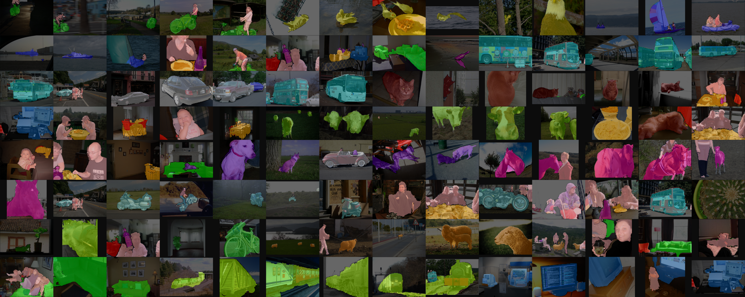
(Refined) Pseudo Segmentation Maps P-NOC +C²AM-H
Figure 47: Pseudo segmentation maps obtained by random walking over segmentation priors generated by a model trained with P-NOC proposals. The Affinity Network was trained over labels refined with saliency maps devised from C²AM-H.
Qualitative Results over VOC 2012 P-NOC +C²AM-H
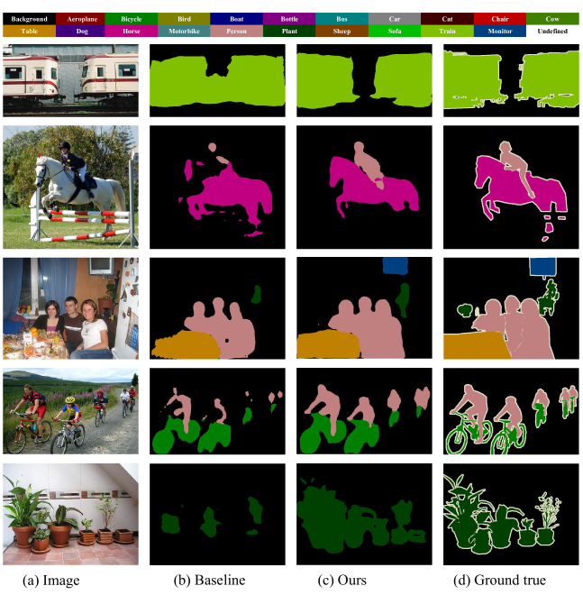
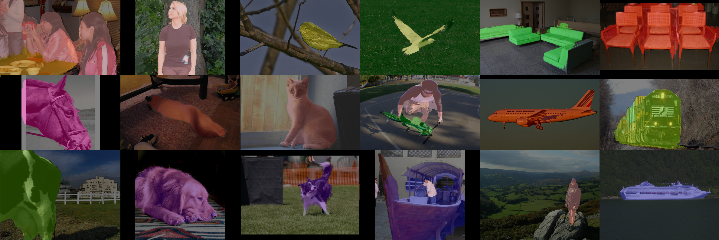
Figure 48: Qualitative results over Pascal VOC 2012 datasets. Segmentation proposals obtained by a DeepLabV3+ model trained with pseudo labels devised from P-NOC +C²AM-H.
Quantitative Results over VOC 2012 P-NOC +C²AM-H
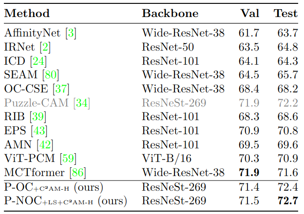
Table 5: Comparison with other methods in literature. mIoU (%) scores are reported for both Pascal VOC 2012 validation and testing sets.
Quantitative Results over COCO 2014 P-NOC +C²AM-H
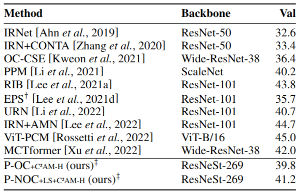
Table 5: Comparison with other methods in literature. mIoU (%) scores are reported for MS COCO 2014 validation set. P-NOC and OC-CSE: priors employed, no refinement conducted.
Schedule
1. Introduction
2. Related Work
3. Research Proposal
4. Preliminary Results
5. Final Considerations
Final Considerations
We conducted studies over:
- XAI in broader (multi-label) scenarios
- MinMax-CAM
- Complementary Regularization Strategies in WSSS
- Adversarial CAM generation for more robust priors
As future work, we propose to:
- Transformers in WSSS
- WSSS in Boundary and Difficult Scenarios
- Ensemble and meta-learning strategies in WSSS
Scientific Production Final Considerations
- L. David, H. Pedrini, and Z. Dias. MinMax-CAM: Improving focus of CAM-based visualization techniques in multi-label problems. In 17th International Joint Conference on Computer Vision, Imaging and Computer Graphics Theory and Applications (VISAPP), pages 106–117. INSTICC, SciTePress, 2022.
- L. David, H. Pedrini, and Z. Dias. MinMax-CAM: Increasing Precision of Explaining Maps by Contrasting Gradient Signals and Regularizing Kernel Usage (Springer). In 17th International Joint Conference on Computer Vision, Imaging and Computer Graphics Theory and Applications (VISAPP), CCIS Series, 2023.
- L. David, H. Pedrini, and Z. Dias. Not so Ordinary Classifier: Revisiting Complementary Regularizing Strategies for More Robust Priors in Weakly Supervised Semantic Segmentation.
Technical Contributions Final Considerations
- Implement pixel ignoring functionality in the cross-entropy loss in Keras, for semantic segmentation problems².
- Ported the Wide ResNet38-d and ResNeSt architectures, originally trained in PyTorch, to TensorFlow.
- Created the keras-explainable library, containing out-of-the box implementations of many Explainable AI algorithms.
- Various fixes in Keras and TensorFlow-Addons, often related to the optimizer, mixed-precision when training in a Multi-Worker-Mirrored-Strategy environment.

