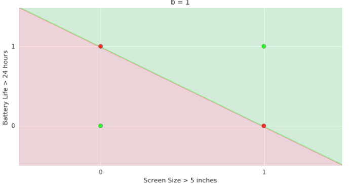
1.6 The Perceptron Model
Your first model with weights
Recap: MP Neuron
What did we see in the previous chapter?
(c) One Fourth Labs
| Screen size (>5 in) | 1 | 0 | 1 | 1 | 1 | 0 | 1 | 0 | 1 | 0 |
| Battery (>2000mAh) | 0 | 0 | 0 | 1 | 0 | 1 | 1 | 1 | 1 | 0 |
| Like | 1 | 0 | 1 | 0 | 1 | 1 | 0 | 1 | 0 | 0 |
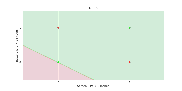


Boolean inputs
Boolean output
Linear
Fixed Slope
Few possible intercepts (b's)
The Road Ahead
What's going to change now ?
(c) One Fourth Labs
Show the six jars and convey the following by animation
-- Boolean inputs gets replaced by real inputs
-- Only one parameter b by "weights for every input" (below model jar)
-- Brute force by "our first learning algorithm"
-- Add Perceptron loss function with a saddie (not smiley)
Linear
Only one parameter, b
Real inputs
Boolean output
Brute force
The Road Ahead
What's going to change now ?
(c) One Fourth Labs
\( \{0, 1\} \)
Boolean


Loss
Model
Data
Task
Evaluation
Learning
Linear
Only one parameter, b
Real inputs
Boolean output
Brute force
Boolean inputs
Our 1st learning algorithm
Weights for every input
Data and Task
What kind of data and tasks can Perceptron process ?
(c) One Fourth Labs
Same data matrix from before with binary inputs and outputs
Animation:
- Now replace some boolean inputs by real inputs (for example, >5in will get replaced by actual screen size, >24 hours will get replaced by actual battery life and so on
- Now, highlight some columns which may seem more important than others (I will just speak through it to say that some features are more important than others
Real inputs
Data and Task
What kind of data and tasks can Perceptron process ?
(c) One Fourth Labs
Real inputs
| Launch (within 6 months) | 0 | 1 | 1 | 0 | 0 | 1 | 0 | 1 | 1 |
| Weight (g) | 151 | 180 | 160 | 205 | 162 | 182 | 138 | 185 | 170 |
| Screen size (inches) | 5.8 | 6.18 | 5.84 | 6.2 | 5.9 | 6.26 | 4.7 | 6.41 | 5.5 |
| dual sim | 1 | 1 | 0 | 0 | 0 | 1 | 0 | 1 | 0 |
| Internal memory (>= 64 GB, 4GB RAM) | 1 | 1 | 1 | 1 | 1 | 1 | 1 | 1 | 1 |
| NFC | 0 | 1 | 1 | 0 | 1 | 0 | 1 | 1 | 1 |
| Radio | 1 | 0 | 0 | 1 | 1 | 1 | 0 | 0 | 0 |
| Battery(mAh) | 3060 | 3500 | 3060 | 5000 | 3000 | 4000 | 1960 | 3700 | 3260 |
| Price (INR) | 15k | 32k | 25k | 18k | 14k | 12k | 35k | 42k | 44k |
| Like (y) | 1 | 0 | 1 | 0 | 1 | 1 | 0 | 1 | 0 |
| Launch (within 6 months) | 0 | 1 | 1 | 0 | 0 | 1 | 0 | 1 | 1 |
| Weight (<160g) | 1 | 0 | 1 | 0 | 0 | 0 | 1 | 0 | 0 |
| Screen size (<5.9 in) | 1 | 0 | 1 | 0 | 1 | 0 | 1 | 0 | 1 |
| dual sim | 1 | 1 | 0 | 0 | 0 | 1 | 0 | 1 | 0 |
| Internal memory (>= 64 GB, 4GB RAM) | 1 | 1 | 1 | 1 | 1 | 1 | 1 | 1 | 1 |
| NFC | 0 | 1 | 1 | 0 | 1 | 0 | 1 | 1 | 1 |
| Radio | 1 | 0 | 0 | 1 | 1 | 1 | 0 | 0 | 0 |
| Battery(>3500mAh) | 0 | 0 | 0 | 1 | 0 | 1 | 0 | 1 | 0 |
| Price > 20k | 0 | 1 | 1 | 0 | 0 | 0 | 1 | 1 | 1 |
| Like (y) | 1 | 0 | 1 | 0 | 1 | 1 | 0 | 1 | 0 |
Data Preparation
Can the data be used as it is ?
(c) One Fourth Labs
Same data matrix from before with binary inputs and outputs
Animation:
- Highlight two columns which have very different ranges (say price and battery life)
- These columns are not comparable
- Now show one of the columns on the RHS
- Highlight the max and min values of this column
- Now show the standardized version of this column
- Repeat this for another column
- FInally replace this matrix by a standardized matrix
(Its ok if you need to do all of this over multiple slides)
Column1
Show one of the columns here
Standardized column
Now show the standardized value of the column here.
Show the computtaions
(x-min)/ (max - min)
(c) One Fourth Labs
| Launch (within 6 months) | 0 | 1 | 1 | 0 | 0 | 1 | 0 | 1 | 1 |
| Weight (g) | 151 | 180 | 160 | 205 | 162 | 182 | 138 | 185 | 170 |
| Screen size (inches) | 5.8 | 6.18 | 5.84 | 6.2 | 5.9 | 6.26 | 4.7 | 6.41 | 5.5 |
| dual sim | 1 | 1 | 0 | 0 | 0 | 1 | 0 | 1 | 0 |
| Internal memory (>= 64 GB, 4GB RAM) | 1 | 1 | 1 | 1 | 1 | 1 | 1 | 1 | 1 |
| NFC | 0 | 1 | 1 | 0 | 1 | 0 | 1 | 1 | 1 |
| Radio | 1 | 0 | 0 | 1 | 1 | 1 | 0 | 0 | 0 |
| Battery(mAh) | 3060 | 3500 | 3060 | 5000 | 3000 | 4000 | 1960 | 3700 | 3260 |
| Price (INR) | 15k | 32k | 25k | 18k | 14k | 12k | 35k | 42k | 44k |
| Like (y) | 1 | 0 | 1 | 0 | 1 | 1 | 0 | 1 | 0 |
| screen size |
|---|
| 5.8 |
| 6.18 |
| 5.84 |
| 6.2 |
| 5.9 |
| 6.26 |
| 4.7 |
| 6.41 |
| 5.5 |
| screen size |
|---|
| 0.64 |
| 0.87 |
| 0.67 |
| 0.88 |
| 0.7 |
| 0.91 |
| 0 |
| 1 |
| 0.47 |
min
max
Standardization formula
| Launch (within 6 months) | 0 | 1 | 1 | 0 | 0 | 1 | 0 | 1 | 1 |
| Weight (g) | 151 | 180 | 160 | 205 | 162 | 182 | 138 | 185 | 170 |
| Screen size | 0.64 | 0.87 | 0.67 | 0.88 | 0.7 | 0.91 | 0 | 1 | 0.47 |
| dual sim | 1 | 1 | 0 | 0 | 0 | 1 | 0 | 1 | 0 |
| Internal memory (>= 64 GB, 4GB RAM) | 1 | 1 | 1 | 1 | 1 | 1 | 1 | 1 | 1 |
| NFC | 0 | 1 | 1 | 0 | 1 | 0 | 1 | 1 | 1 |
| Radio | 1 | 0 | 0 | 1 | 1 | 1 | 0 | 0 | 0 |
| Battery(mAh) | 3060 | 3500 | 3060 | 5000 | 3000 | 4000 | 1960 | 3700 | 3260 |
| Price (INR) | 15k | 32k | 25k | 18k | 14k | 12k | 35k | 42k | 44k |
| Like (y) | 1 | 0 | 1 | 0 | 1 | 1 | 0 | 1 | 0 |
| battery |
|---|
| 3060 |
| 3500 |
| 3060 |
| 5000 |
| 3000 |
| 4000 |
| 1960 |
| 3700 |
| 3260 |
| battery |
|---|
| 0.36 |
| 0.51 |
| 0.36 |
| 1 |
| 0.34 |
| 0.67 |
| 0 |
| 0.57 |
| 0.43 |
min
max
Data Preparation
Can the data be used as it is ?
| Launch (within 6 months) | 0 | 1 | 1 | 0 | 0 | 1 | 0 | 1 | 1 |
| Weight (g) | 151 | 180 | 160 | 205 | 162 | 182 | 138 | 185 | 170 |
| Screen size | 0.64 | 0.87 | 0.67 | 0.88 | 0.7 | 0.91 | 0 | 1 | 0.47 |
| dual sim | 1 | 1 | 0 | 0 | 0 | 1 | 0 | 1 | 0 |
| Internal memory (>= 64 GB, 4GB RAM) | 1 | 1 | 1 | 1 | 1 | 1 | 1 | 1 | 1 |
| NFC | 0 | 1 | 1 | 0 | 1 | 0 | 1 | 1 | 1 |
| Radio | 1 | 0 | 0 | 1 | 1 | 1 | 0 | 0 | 0 |
| Battery | 0.36 | 0.51 | 0.36 | 1 | 0.34 | 0.67 | 0 | 0.57 | 0.43 |
| Price (INR) | 15k | 32k | 25k | 18k | 14k | 12k | 35k | 42k | 44k |
| Like (y) | 1 | 0 | 1 | 0 | 1 | 1 | 0 | 1 | 0 |
Data Preparation
Can the data be used as it is ?
(c) One Fourth Labs
| Launch (within 6 months) | 0 | 1 | 1 | 0 | 0 | 1 | 0 | 1 | 1 |
| Weight | 0.19 | 0.63 | 0.33 | 1 | 0.36 | 0.66 | 0 | 0.70 | 0.48 |
| Screen size | 0.64 | 0.87 | 0.67 | 0.88 | 0.7 | 0.91 | 0 | 1 | 0.47 |
| dual sim | 1 | 1 | 0 | 0 | 0 | 1 | 0 | 1 | 0 |
| Internal memory (>= 64 GB, 4GB RAM) | 1 | 1 | 1 | 1 | 1 | 1 | 1 | 1 | 1 |
| NFC | 0 | 1 | 1 | 0 | 1 | 0 | 1 | 1 | 1 |
| Radio | 1 | 0 | 0 | 1 | 1 | 1 | 0 | 0 | 0 |
| Battery | 0.36 | 0.51 | 0.36 | 1 | 0.34 | 0.67 | 0 | 0.57 | 0.43 |
| Price | 0.09 | 0.63 | 0.41 | 0.19 | 0.06 | 0 | 0.72 | 0.94 | 1 |
| Like (y) | 1 | 0 | 1 | 0 | 1 | 1 | 0 | 1 | 0 |
| Launch (within 6 months) | 0 | 1 | 1 | 0 | 0 | 1 | 0 | 1 | 1 |
| Weight (g) | 151 | 180 | 160 | 205 | 162 | 182 | 138 | 185 | 170 |
| Screen size (inches) | 0.64 | 0.87 | 0.67 | 0.88 | 0.7 | 0.91 | 0 | 1 | 0.47 |
| dual sim | 1 | 1 | 0 | 0 | 0 | 1 | 0 | 1 | 0 |
| Internal memory (>= 64 GB, 4GB RAM) | 1 | 1 | 1 | 1 | 1 | 1 | 1 | 1 | 1 |
| NFC | 0 | 1 | 1 | 0 | 1 | 0 | 1 | 1 | 1 |
| Radio | 1 | 0 | 0 | 1 | 1 | 1 | 0 | 0 | 0 |
| Battery(mAh) | 0.36 | 0.51 | 0.36 | 1 | 0.34 | 0.67 | 0 | 0.57 | 0.43 |
| Price (INR) | 15k | 32k | 25k | 18k | 14k | 12k | 35k | 42k | 44k |
| Like (y) | 1 | 0 | 1 | 0 | 1 | 1 | 0 | 1 | 0 |
| weight |
|---|
| 0.19 |
| 0.63 |
| 0.33 |
| 1 |
| 0.36 |
| 0.66 |
| 0 |
| 0.70 |
| 0.48 |
| battery |
|---|
| 0.36 |
| 0.51 |
| 0.36 |
| 1 |
| 0.34 |
| 0.67 |
| 0 |
| 0.57 |
| 0.43 |
| price |
|---|
| 0.09 |
| 0.63 |
| 0.41 |
| 0.19 |
| 0.06 |
| 0 |
| 0.72 |
| 0.94 |
| 1 |
| Launch (within 6 months) | 0 | 1 | 1 | 0 | 0 | 1 | 0 | 1 | 1 |
| Weight (g) | 151 | 180 | 160 | 205 | 162 | 182 | 138 | 185 | 170 |
| Screen size (inches) | 0.64 | 0.87 | 0.67 | 0.88 | 0.7 | 0.91 | 0 | 1 | 0.47 |
| dual sim | 1 | 1 | 0 | 0 | 0 | 1 | 0 | 1 | 0 |
| Internal memory (>= 64 GB, 4GB RAM) | 1 | 1 | 1 | 1 | 1 | 1 | 1 | 1 | 1 |
| NFC | 0 | 1 | 1 | 0 | 1 | 0 | 1 | 1 | 1 |
| Radio | 1 | 0 | 0 | 1 | 1 | 1 | 0 | 0 | 0 |
| Battery(mAh) | 0.36 | 0.51 | 0.36 | 1 | 0.34 | 0.67 | 0 | 0.57 | 0.43 |
| Price (INR) | 15k | 32k | 25k | 18k | 14k | 12k | 35k | 42k | 44k |
| Like (y) | 1 | 0 | 1 | 0 | 1 | 1 | 0 | 1 | 0 |
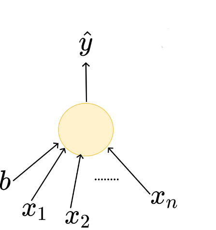
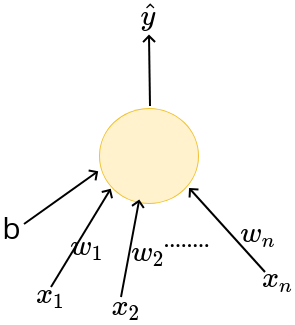
The Model
What is the mathematical model ?
(c) One Fourth Labs
Show the standardised data matrix
Show the model here
The Model
What is the mathematical model ?
(c) One Fourth Labs
| Launch (within 6 months) | 0 | 1 | 1 | 0 | 0 | 1 | 0 | 1 | 1 |
| Weight | 0.19 | 0.63 | 0.33 | 1 | 0.36 | 0.66 | 0 | 0.70 | 0.48 |
| Screen size | 0.64 | 0.87 | 0.67 | 0.88 | 0.7 | 0.91 | 0 | 1 | 0.47 |
| dual sim | 1 | 1 | 0 | 0 | 0 | 1 | 0 | 1 | 0 |
| Internal memory (>= 64 GB, 4GB RAM) | 1 | 1 | 1 | 1 | 1 | 1 | 1 | 1 | 1 |
| NFC | 0 | 1 | 1 | 0 | 1 | 0 | 1 | 1 | 1 |
| Radio | 1 | 0 | 0 | 1 | 1 | 1 | 0 | 0 | 0 |
| Battery | 0.36 | 0.51 | 0.36 | 1 | 0.34 | 0.67 | 0 | 0.57 | 0.43 |
| Price | 0.09 | 0.63 | 0.41 | 0.19 | 0.06 | 0 | 0.72 | 0.94 | 1 |
| Like (y) | 1 | 0 | 1 | 0 | 1 | 1 | 0 | 1 | 0 |
\(x_1\)
b
\(x_n\)
\(\hat{y}\)
\(x_2\)
\(w_1\)
\(w_2\)
\(w_n\)
The Model
How is this different from the Perceptron Model ?
(c) One Fourth Labs
1) Show the equations side by side of MP and perceptron and see what is changing
Real inputs
Linear
Weights for each input
Adjustable threshold
Boolean inputs
Linear
Inputs are not weighted
Adjustable threshold
The Model
How is this different from the Perceptron Model ?
(c) One Fourth Labs
Real inputs
Linear
Weights for each input
Adjustable threshold
Boolean inputs
Linear
Inputs are not weighted
Adjustable threshold
The Model
What do weights allow us to do ?
(c) One Fourth Labs
Hard part: the examples mentioned below need to be constructed carefully
- Show two examples where all features are same but one has high price (no_buy) and the other has low price (buy)
- 9 terms in the sum will be same
- now if there is a negative weight attached with the price then one will cross the threshold and the other will not
- weights can be inhibitory (negative) or excitatory (positive)
Show standardised data from before. Focus on price and output and show that there is an inverse relation between them.
The Model
What do weights allow us to do ?
(c) One Fourth Labs
| Launch (within 6 months) | 0 | 1 | 1 | 0 | 0 | 1 | 0 | 1 | 1 |
| Weight (g) | 151 | 180 | 160 | 205 | 162 | 182 | 138 | 185 | 170 |
| Screen size (inches) | 5.8 | 6.18 | 5.84 | 6.2 | 5.9 | 6.26 | 4.7 | 6.41 | 5.5 |
| dual sim | 1 | 1 | 0 | 0 | 0 | 1 | 0 | 1 | 0 |
| Internal memory (>= 64 GB, 4GB RAM) | 1 | 1 | 1 | 1 | 1 | 1 | 1 | 1 | 1 |
| NFC | 0 | 1 | 1 | 0 | 1 | 0 | 1 | 1 | 1 |
| Radio | 1 | 0 | 0 | 1 | 1 | 1 | 0 | 0 | 0 |
| Battery(mAh) | 3060 | 3500 | 3060 | 5000 | 3000 | 4000 | 1960 | 3700 | 3260 |
| Price (INR) | 15k | 32k | 25k | 18k | 14k | 12k | 35k | 42k | 44k |
| Like (y) | 1 | 0 | 1 | 0 | 1 | 1 | 0 | 1 | 0 |
\(x_1\)
b
\(x_n\)
\(\hat{y}\)
\(x_2\)
\(w_1\)
\(w_2\)
\(w_n\)
\(w_{price} \rightarrow -ve\)
Like \(\alpha \frac{1}{price}\)
Some Math fundae
Can we write the perceptron model slightly more compactly?
(c) One Fourth Labs
|
Some Math fundae
Can we write the perceptron model slightly more compactly?
(c) One Fourth Labs
x : [0, 0.19, 0.64, 1, 1, 0]
w: [0.3, 0.4, -0.3, 0.1, 0.5]
\(\vec{x} \in R^5\)
\(\vec{w} \in R^5\)
\( \vec{x} \)
\( \vec{w} \)
\(\vec{x}.\vec{w}\) = ?
\(\vec{x}.\vec{w} = x_1.w_1 + x_2.w_2 + ... x_n.w_n\)
\(x_1\)
b
\(x_n\)
\(\hat{y}\)
\(x_2\)
\(w_1\)
\(w_2\)
\(w_n\)
The Model
What is the geometric interpretation of the model ?
(c) One Fourth Labs
- On LHS again recap the two variable plot for perceptron
- show how the green and red half planes change as b=0,1,2
- Read the remaining slides also before making this slide so that you can have a meaningful example throughout
- On RHS show the same plot and show that now in the case of perceptron, for a given value of b we can also rotate the line by changing the slope w. and get multiple partitions of green and red half planes
- Also show that b itself is smooth now and not restricted to values 0,1, and 2
More freedom
The Model
Why is more freedom important ?
(c) One Fourth Labs
- Plot some data with two variables x1 and x2 such that the positive and negative points cannot be separated by MP model but can be separated by the perceptron model
More freedom
The Model
Is this all the freedom that we need ?
(c) One Fourth Labs
- On LHS show a perceptron type data plot where it is impossible to drawn any line to separate the positive points from the negative points.
- For example, in the case of phone think of two features such that it is fine if either of them is present but not if both are present
- Show that we will need a complex decision surface to divide the green and red points. Take a surface such that you can write an equation for it so that we can show that instead of line we now need this complex function
We want even more freedom
- on RHS show a data plot where there are some outliers within positive and negative clusters
- Now show a complex surface such that we can separate the positive and negative points completely
- Now show even more complex outliers and show you need even more complex surfaces (somewhat similar to Andrej Karpathy's plot which we have used to explain adversarial examples in the lecture on Visualize CNNs)
The Model
What if we have more than 2 dimensions ?
(c) One Fourth Labs
- Now show a 3d plot and show how in 3d also perceptron still divides the input space into two halves - red and blue
- I would like to have an animation which shows that as we change w_1, w_2 and b how the plane changes
- now on RHS show one more plot here have you have some data which cannot be separated by a plane and no matter how you adjust w_1, w_2 and b you cannot separate these points
- Again, this can be done by apparently creating a video from python itself. You can ask Harish (check with Ananya) to do this
Inference
How do you put this model to use ?
(c) One Fourth Labs
1. Show small training matrix here
2. Show humans with rules in his head
3. Show show one test instance here
4. Show human's output here
5 - now replace human with perceptron model and
6 - now replace human's output with model equations and compute the output
Loss Function
What is the loss function that you use for this model ?
(c) One Fourth Labs
First write it as this,
L = 0 if y = \hat{y}
= 1 if y != \hat{y}
Now write it more compactly as
\indicator_{y - \hat{y}}
1. Show small training matrix here
2. Show the loss function as if-else
3. Show the loss function as indicator variable
4. Now add a column for y_hat and compute the loss
5. Now show the pink box with the QA
Q. What is the purpose of the loss function ?
A. To tell the model that some correction needs to be done!
Q. How ?
A. We will see soon
Loss Function
What is the loss function that you use for this model ?
(c) One Fourth Labs
| Weight | Screen size | Like |
|---|---|---|
| 0.19 | 0.64 | 1 |
| 0.63 | 0.87 | 1 |
| 0.33 | 0.67 | 0 |
| 1 | 0.88 | 0 |
| Weight | Screen size | Like | Loss | |
|---|---|---|---|---|
| 0.19 | 0.64 | 1 | 1 | 0 |
| 0.63 | 0.87 | 1 | 0 | 1 |
| 0.33 | 0.67 | 0 | 1 | 1 |
| 1 | 0.88 | 0 | 0 | 0 |
Q. What is the purpose of the loss function ?
A. To tell the model that some correction needs to be done!
Q. How ?
A. We will see soon
Loss Function
How is this different from the squared error loss function ?
(c) One Fourth Labs
First write it as this,
L = 0 if y = \hat{y}
= 1 if y != \hat{y}
Now write it more compactly as
\indicator_{y - \hat{y}}
1. Show small training matrix here
2. Show the loss function as if-else
3. Show the loss function as indicator variable
4. Now add a column for y_hat and compute the loss
5. Now show the pink box with the QA
Q. What is the purpose of the loss function ?
A. To tell the model that some correction needs to be done!
Q. How ?
A. We will see soon
Loss Function
How is this different from the squared error loss function ?
(c) One Fourth Labs
1.
Show small training matrix here
Show output of model
2. squared error loss and perceptron loss formula on LHS
3. Add two columns to compute these losses one row at a time the QA
4 Show the pink box
Squared error loss is equivalent to perceptron loss when the outputs are boolean
Loss Function
How is this different from the squared error loss function ?
(c) One Fourth Labs
Squared error loss is equivalent to perceptron loss when the outputs are boolean.
| Weight | Screen size | Like | |
|---|---|---|---|
| 0.19 | 0.64 | 1 | 1 |
| 0.63 | 0.87 | 1 | 0 |
| 0.33 | 0.67 | 0 | 1 |
| 1 | 0.88 | 0 | 0 |
| Perceptron Loss | Squared Error Loss |
|---|---|
0
0
0
0
1
1
1
1
Perceptron loss =
Squared Error loss =
Loss Function
Can we plot the loss function ?
(c) One Fourth Labs
- Show single variable data on LHS so that there are only two parameters w,b
- Show model below it
- Now show a 3d-plot with w,b,error
- Substitute different values of w,b and compute output (additional column in the matrix) and loss (additional column in the matrix)
- Show how the error changes as you change the value of w,b
| Weight | Like |
|---|---|
| 0.19 | 1 |
| 0.63 | 0 |
| 0.33 | 1 |
| 1 | 0 |
\(w_1\)
\(x_1\)
\(\hat{y}\)
b
Learning Algorithm
What is the typical recipe for learning parameters of a model ?
(c) One Fourth Labs
Initialise
1. Show training matrix with 2 inouts and one output
2. on LHS show the box containing w1, w2, b
3. Initialize
4. Iterate over data
5. Highlight first row in data
6. compute_loss
7. update
8 now highlight iterate over data
9. highlight second row, third row, ..., come back to first row
10. till satisfied
11. replace w1, w2 by w and show the box below
\(w_1, w_2, b \)
Iterate over data:
\( \mathscr{L} = compute\_loss(x_i) \)
\( update(w_1, w_2, b, \mathscr{L}) \)
till satisfied
\(\mathbf{w} = [w_1, w_2] \)
Learning Algorithm
What does the perceptron learning algorithm look like ?
Show the algorithm here, use similar animations as in my lecture. I don't think you can use \algorithmic here
Instead of defining P and N, you can just rewrite the "if" condition as "if y_i = 1 and wx < 0"
w = w + x
b = b + 1
Show the model equation here
First in summation form and then in vector form
Show that the input x is also a vector
(c) One Fourth Labs
Learning Algorithm
Can we see this algorithm in action ?
(c) One Fourth Labs
Show the data here
Add a column for wx+b
and a column for y_hat
Show the algorithm here
Show a 3d plot here of how the values of w1,w2 and b change and the positive and negative half space changes as you go over each data point
Learning Algorithm
What is the geometric interpretation of this ?
(c) One Fourth Labs
- Show model equations again
- Now show the plot and the animations suggested in the black box on the RHS
Now show a plot containing only w and b
show what happens when we do b = b + 1. (The line shifts towards the point)
show what happens when we do w = w + x
(the line rotates towards the point)
Repeat the same for a negative point and show that the opposite happens
Learning Algorithm
What is the geometric interpretation of this (in higher dimensions) ?
(c) One Fourth Labs
- Show model equations again
- Now drop b from the equation
- wx = 0 is a plane which separates the input space into two halves (show plane in the plot)
- Every point x on this plane satisfies the equation wx = 0 (show a plane and points on this plane as vectors)
- w is perpendicular to this plane (show w vector perpendicular to all the points and hence the plane )
- Now show a point in the positive half space as a vector
- Show angle \alpha between this vector and the w vector
- below this box \alpha < 90 --> cos \alpha <0 --> wx < 0
- repeat the above for a negative point
Plot here
Learning Algorithm
How does adding/subtracting x to/from w help ?
(c) One Fourth Labs
Highlight a negative point which was misclassified (you will have to show that it lies on the other side of the plane)
cos(\aplha) = wx < 0
w_new = w - x
cos(\apha_new) = ...now the derivation from my lecture slides
now show that the plane indeed rotates so that the point moves closer to the negative half space (there is a continuation on the next slide)
Plot here
Learning Algorithm
How does adding/subtracting 1 from b help ?
(c) One Fourth Labs
b = b - 1
the plane will move down now so that the point will go to the other side
Plot here
Learning Algorithm
Will this algorithm always work ?
(c) One Fourth Labs
Show a plot of linearly separable data (similar to that in my lecture slides)
Now draw a line which separates the points
Show a plot of linearly separable data (similar to that in my lecture slides)
Now draw a line which separates the points
Only if the data is linearly separable
Learning Algorithm
Can we prove that it will always work for linearly separable data ?
(c) One Fourth Labs
Show a plot of linearly separable data (similar to that in my lecture slides)
Now draw a line which separates the points
Put the statement of the proof here
Learning Algorithm
What does "till satisfied" mean ?
(c) One Fourth Labs
Initialise
\(w_1, w_2, b \)
Iterate over data:
\( \mathscr{L} = compute\_loss(x_i) \)
\( update(w_1, w_2, b, \mathscr{L}) \)
till satisfied
\( total\_loss = 0 \)
\( total\_loss += \mathscr{L} \)
till total loss becomes 0
till total loss becomes < \( \epsilon \)
till number of iterations exceeds k (say 100)
Evaluation
How do you check the performance of the perceptron model?
(c) One Fourth Labs
Same slide as that in MP neuron
Take-aways
So will you use MP neuron?
(c) One Fourth Labs
Show the 6 jars at the top (again can be small)
\( \{0, 1\} \)
\( \in \mathbb{R} \)
Boolean
show the line plot with the issue of non-linearly separable data
show squared error loss
show perceptronlearning algorithm
show accuracy formula
An Eye on the Capstone project
How is perceptron related to the capstone project ?
(c) One Fourth Labs
Show the 6 jars at the top (again can be small)
\( \{0, 1\} \)
\( \in \mathbb{R} \)
Show that the signboard image can be represented as real numbers
Boolean
text/no-text
Show a plot with all text images on one side and non-text on another
show squared error loss
show perceptronlearning algorithm
show accuracy formula
and show a small matrix below with some ticks and crossed and show how accuracy will be calculated
The simplest model for binary classification
\( \{0, 1\} \)
Boolean
Loss
Model
Data
Task
Evaluation
Learning
Linear
Only one parameter, b
Real inputs
Boolean output
Brute force
Boolean inputs
Our 1st learning algorithm
Weights for every input
Assignments
How do you view the learning process ?
(c) One Fourth Labs
Assignment: Give some data including negative values and ask them to standardize it