Python for AI/ML/Data Science 自修心得

0. ML 入門

1. Datacamp "Deep Learning in Python" 最容易入門

2. Data Science from Scratch

- First Principles with Python by Joel Grus

(if related to ML, for generic Python related, check another deck in Self learning - Python)

3. Keras

4. Google Colab - Python Programming 4 ML from Scratch

4/6/2018

about me

EE degree back in 1982

Z80 was the most popular CPU

Pascal/Fortran/COBOL were popular languages

Apple ][ + BASIC and CP/M

intel 80386SX PC mother board designer

......

Interested in Linux since 2016

Z80 CPU

intel 80386SX CPU

photo source: wikipedia.org

Apple ][

marconi.jiang@gmail.com

參考資料

Code for the book on GitHub

Vocaburary

Text

Layman Terms for Machine Learning

Machine Learning / Deep Learning 因為 Google Alpha Go 於2016年3月8日到3月15日在南韓首爾舉行打敗韓國圍棋高手李世AlphaGo對李世乭是由韓國職業九段棋士李世乭

2. Datacamp "Deep Learning in Python"

5/7/2018

introduction to Deep Learning

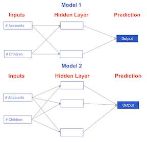
Comparing neural network models to classical regression models

Which of the models in the diagrams has greater ability to account for interactions?

Forward Propagation

Example 1.1.1 說明

Coding the forward propagation algorithm

In this exercise, you'll write code to do forward propagation (prediction) for your first neural network:

Ch1Ex4

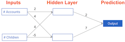
Each data point is a customer. The first input is how many accounts they have, and the second input is how many children they have. The model will predict how many transactions the user makes in the next year. You will use this data throughout the first 2 chapters of this course.

The input data has been pre-loaded as input_data, and the weights are available in a dictionary called weights. The array of weights for the first node in the hidden layer are in weights['node_0'], and the array of weights for the second node in the hidden layer are in weights['node_1'].

The weights feeding into the output node are available in weights['output'].

NumPy will be pre-imported for you as np in all exercises.

Example 1.1.1 說明

Example 1.1.1

import numpy as np

input_data =np.array([2,3])
weights = {'node_0': np.array([1, 1]), 
           'node_1': np.array([-1, 1]), 
           'output': np.array([2, -1])}

# Calculate node 0 value: node_0_value
node_0_value = (input_data * weights['node_0']).sum()

# Calculate node 1 value: node_1_value
node_1_value = (input_data * weights['node_1']).sum()

# Put node values into array: hidden_layer_outputs
hidden_layer_outputs = np.array([node_0_value, node_1_value])

# Calculate output: output
output = (hidden_layer_outputs * weights['output']).sum()

# Print output
print(output)

Activation Function

Example 1.1.2 說明

The Rectified Linear Activation Function

As Dan explained to you in the video, an "activation function" is a function applied at each node. It converts the node's input into some output.

The rectified linear activation function (called ReLU) has been shown to lead to very high-performance networks. This function takes a single number as an input, returning 0 if the input is negative, and the input if the input is positive.

Here are some examples:
relu(3) = 3
relu(-3) = 0

Example 1.1.2 說明

SCRIPT.PY

Example 1.1.2

def relu(input):
    '''Define your relu activation function here'''
    # Calculate the value for the output of the relu function: output
    output = max(input, 0)
    
    # Return the value just calculated
    return(output)

# Calculate node 0 value: node_0_output
node_0_input = (input_data * weights['node_0']).sum()
node_0_output = relu(node_0_input)

# Calculate node 1 value: node_1_output
node_1_input = (input_data * weights['node_1']).sum()
node_1_output = relu(node_1_input)

# Put node values into array: hidden_layer_outputs
hidden_layer_outputs = np.array([node_0_output, node_1_output])

# Calculate model output (do not apply relu)
model_output = (hidden_layer_outputs * weights['output']).sum()

# Print model output
print(model_output)

Example 1.1.3 說明

Applying the network to many observations/rows of data

You'll now define a function called predict_with_network()which will generate predictions for multiple data observations, which are pre-loaded as input_data. As before, weightsare also pre-loaded. In addition, the relu() function you defined in the previous exercise has been pre-loaded.

Example 1.1.3 說明

Define a function called predict_with_network() that accepts two arguments - input_data_row and weights - and returns a prediction from the network as the output.
Calculate the input and output values for each node, storing them as: node_0_input, node_0_output, node_1_input, and node_1_output.
- To calculate the input value of a node, multiply the relevant arrays together and compute their sum.
- To calculate the output value of a node, apply the relu()function to the input value of the node.
Use a for loop to iterate over input_data:
- Use your predict_with_network() to generate predictions for each row of the input_data - input_data_row. Append each prediction to results.

Take Hint (-30 XP)

Example 1.1.3

# Define predict_with_network()
def predict_with_network(input_data_row, weights):

    # Calculate node 0 value
    node_0_input = (input_data_row * weights['node_0']).sum()
    node_0_output = relu(node_0_input)

    # Calculate node 1 value
    node_1_input = (input_data_row * weights['node_1']).sum()
    node_1_output = relu(node_1_input)

    # Put node values into array: hidden_layer_outputs
    hidden_layer_outputs = np.array([node_0_output, node_1_output])
    
    # Calculate model output
    input_to_final_layer = (hidden_layer_outputs * weights['output']).sum()
    model_output = relu(input_to_final_layer)
    
    # Return model output
    return(model_output)


# Create empty list to store prediction results
results = []
for input_data_row in input_data:
    # Append prediction to results
    results.append(predict_with_network(input_data_row, weights))

# Print results
print(results)

Deeper Network

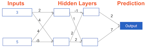
Forward propagation in a deeper network

You now have a model with 2 hidden layers. The values for an input data point are shown inside the input nodes. The weights are shown on the edges/lines. What prediction would this model make on this data point?

Assume the activation function at each node is the identity function. That is, each node's output will be the same as its input. So the value of the bottom node in the first hidden layer is -1, and not 0, as it would be if the ReLU activation function was used.

Example 1.1.4 說明

Multi-layer neural networks

In this exercise, you'll write code to do forward propagation for a neural network with 2 hidden layers. Each hidden layer has two nodes. The input data has been preloaded as input_data. The nodes in the first hidden layer are called node_0_0 and node_0_1. Their weights are pre-loaded as weights['node_0_0'] and weights['node_0_1']respectively.

The nodes in the second hidden layer are called node_1_0and node_1_1. Their weights are pre-loaded as weights['node_1_0'] and weights['node_1_1']respectively.

We then create a model output from the hidden nodes using weights pre-loaded as weights['output'].

Ch1Ex10

Example 1.1.4 說明

SCRIPT.PY

1
2
3
4
5
6
7
8
9
10
11
12
13
14
15
 
 
 

def predict_with_network(input_data):
# Calculate node 0 in the first hidden layer

node_0_0_input = (input_data * weights['node_0_0']).sum()

node_0_0_output = relu(node_0_0_input)
 
# Calculate node 1 in the first hidden layer

node_0_1_input = (input_data * weights['node_0_1']).sum()

node_0_1_output = relu(node_0_1_input)
 
# Put node values into array: hidden_0_outputs

hidden_0_outputs = np.array([node_0_0_output, node_0_1_output])
 
# Calculate node 0 in the second hidden layer

node_1_0_input = (hidden_0_outputs * weights['node_1_0']).sum()
 
 
 

Example 1.1.4

def predict_with_network(input_data):
    # Calculate node 0 in the first hidden layer
    node_0_0_input = (input_data * weights['node_0_0']).sum()
    node_0_0_output = relu(node_0_0_input)

    # Calculate node 1 in the first hidden layer
    node_0_1_input = (input_data * weights['node_0_1']).sum()
    node_0_1_output = relu(node_0_1_input)

    # Put node values into array: hidden_0_outputs
    hidden_0_outputs = np.array([node_0_0_output, node_0_1_output])
    
    # Calculate node 0 in the second hidden layer
    node_1_0_input = (hidden_0_outputs * weights['node_1_0']).sum()
    node_1_0_output = relu(node_1_0_input)

    # Calculate node 1 in the second hidden layer
    node_1_1_input = (hidden_0_outputs * weights['node_1_1']).sum()
    node_1_1_output = relu(node_1_1_input)

    # Put node values into array: hidden_1_outputs
    hidden_1_outputs = np.array([node_1_0_output, node_1_1_output])

    # Calculate model output: model_output
    model_output = (hidden_1_outputs * weights['output']).sum()
    
    # Return model_output
    return(model_output)

output = predict_with_network(input_data)
print(output)

Example 1.1.4

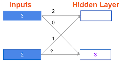
Representations are learned

How are the weights that determine the features/interactions in Neural Networks created?

ANSWER THE QUESTION

50 XP

Possible Answers

A user chooses them when creating the model.

press 1
The model training process sets them to optimize predictive accuracy.

press 2
The weights are random numbers.

press 3

Submit Answer

Take Hint (-15 XP)

Example 1.1.4

Levels of representation

Which layers of a model capture more complex or "higher level" interactions?

ANSWER THE QUESTION

50 XP

Possible Answers

The first layers capture the most complex interactions.

press 1
The last layers capture the most complex interactions.

press 2
All layers capture interactions of similar complexity.

press 3

Submit Answer

Take Hint (-15 XP)

The Needs for Optimization

Chap 2

Calculating model errors

For the exercises in this chapter, you'll continue working with the network to predict transactions for a bank.

What is the error (predicted - actual) for the following network when the input data is [3, 2] and the actual value of the target (what you are trying to predict) is 5? It may be helpful to get out a pen and piece of paper to calculate these values.

Chap 2

Understanding how weights change model accuracy

Imagine you have to make a prediction for a single data point. The actual value of the target is 7. The weight going from node_0 to the output is 2, as shown below. If you increased it slightly, changing it to 2.01, would the predictions become more accurate, less accurate, or stay the same?

Example 2.1.1 說明

Coding how weight changes affect accuracy

Now you'll get to change weights in a real network and see how they affect model accuracy!

Have a look at the following neural network: Ch2Ex4

Its weights have been pre-loaded as weights_0. Your task in this exercise is to update a single weight in weights_0 to create weights_1, which gives a perfect prediction (in which the predicted value is equal to target_actual: 3).

Use a pen and paper if necessary to experiment with different combinations. You'll use the predict_with_network()function, which takes an array of data as the first argument, and weights as the second argument.

Example 2.1.1 說明

Create a dictionary of weights called weights_1 where you have changed 1 weight from weights_0 (You only need to make 1 edit to weights_0 to generate the perfect prediction).
Obtain predictions with the new weights using the predict_with_network() function with input_data and weights_1.
Calculate the error for the new weights by subtracting target_actual from model_output_1.
Hit 'Submit Answer' to see how the errors compare!

Example 2.1.1

# The data point you will make a prediction for
input_data = np.array([0, 3])

# Sample weights
weights_0 = {'node_0': [2, 1],
             'node_1': [1, 2],
             'output': [1, 1]
            }

# The actual target value, used to calculate the error
target_actual = 3

# Make prediction using original weights
model_output_0 = predict_with_network(input_data, weights_0)

# Calculate error: error_0
error_0 = model_output_0 - target_actual

# Create weights that cause the network to make perfect prediction (3): weights_1
weights_1 = {'node_0': [2, 1],
             'node_1': [1, 2],
             'output': [-1, 1]
            }

# Make prediction using new weights: model_output_1
model_output_1 = predict_with_network(input_data, weights_1)

# Calculate error: error_1
error_1 = model_output_1 - target_actual

# Print error_0 and error_1
print(error_0)
print(error_1)

Example 2.1.2 說明

Scaling up to multiple data points

You've seen how different weights will have different accuracies on a single prediction. But usually, you'll want to measure model accuracy on many points. You'll now write code to compare model accuracies for two different sets of weights, which have been stored as weights_0 and weights_1.

input_data is a list of arrays. Each item in that list contains the data to make a single prediction. target_actuals is a list of numbers. Each item in that list is the actual value we are trying to predict.

In this exercise, you'll use the mean_squared_error()function from sklearn.metrics. It takes the true values and the predicted values as arguments.

You'll also use the preloaded predict_with_network()function, which takes an array of data as the first argument, and weights as the second argument.

Example 2.1.2 說明

Import mean_squared_error from sklearn.metrics.
Using a for loop to iterate over each row of input_data:
- Make predictions for each row with weights_0 using the predict_with_network() function and append it to model_output_0.
- Do the same for weights_1, appending the predictions to model_output_1.
Calculate the mean squared error of model_output_0 and then model_output_1 using the mean_squared_error()function. The first argument should be the actual values (target_actuals), and the second argument should be the predicted values (model_output_0 or model_output_1).

Example 2.1.2

from sklearn.metrics import mean_squared_error

# Create model_output_0 
model_output_0 = []
# Create model_output_0
model_output_1 = []


# Loop over input_data
for row in input_data:
    # Append prediction to model_output_0
    model_output_0.append(predict_with_network(row, weights_0))
    
    # Append prediction to model_output_1
    model_output_1.append(predict_with_network(row, weights_1))

# Calculate the mean squared error for model_output_0: mse_0
mse_0 = mean_squared_error(target_actuals, model_output_0)

# Calculate the mean squared error for model_output_1: mse_1
mse_1 = mean_squared_error(target_actuals, model_output_1)

# Print mse_0 and mse_1
print("Mean squared error with weights_0: %f" %mse_0)
print("Mean squared error with weights_1: %f" %mse_1)

Gradient Decent

Example 2.2.1 說明

Calculating slopes

You're now going to practice calculating slopes. When plotting the mean-squared error loss function against predictions, the slope is 2 * x * (y-xb), or 2 * input_data * error. Note that x and b may have multiple numbers (x is a vector for each data point, and b is a vector). In this case, the output will also be a vector, which is exactly what you want.

You're ready to write the code to calculate this slope while using a single data point. You'll use pre-defined weights called weights as well as data for a single point called input_data. The actual value of the target you want to predict is stored in target.

Example 2.2.1 說明

Calculate the predictions, preds, by multiplying weightsby the input_data and computing their sum.
Calculate the error, which is the difference between targetand preds. Notice that this error corresponds to y-xb in the gradient expression.
Calculate the slope of the loss function with respect to the prediction. To do this, you need to take the product of input_data and error and multiply that by 2.

Example 2.2.1

weights = [0, 2, 1]
input_data = [1, 2, 3]
target = 0

# Calculate the predictions: preds
preds = (weights * input_data).sum()

# Calculate the error: error
error = preds - target

# Calculate the slope: slope
slope = 2 * input_data * error

# Print the slope
print(slope)

Example 2.2.2 說明

Improving model weights

Hurray! You've just calculated the slopes you need. Now it's time to use those slopes to improve your model. If you add the slopes to your weights, you will move in the right direction. However, it's possible to move too far in that direction. So you will want to take a small step in that direction first, using a lower learning rate, and verify that the model is improving.

The weights have been pre-loaded as weights, the actual value of the target as target, and the input data as input_data. The predictions from the initial weights are stored as preds.

Example 2.2.2 說明

Set the learning rate to be 0.01 and calculate the error from the original predictions. This has been done for you.
Calculate the updated weights by subtracting the product of learning_rate and slope from weights.
Calculate the updated predictions by multiplying weights_updated with input_data and computing their sum.
Calculate the error for the new predictions. Store the result as error_updated.
Hit 'Submit Answer' to compare the updated error to the original!

Example 2.2.2

# Set the learning rate: learning_rate
learning_rate = 0.01

# Calculate the predictions: preds
preds = (weights * input_data).sum()

# Calculate the error: error
error = preds - target

# Calculate the slope: slope
slope = 2 * input_data * error

# Update the weights: weights_updated
weights_updated = weights - learning_rate * slope

# Get updated predictions: preds_updated
preds_updated = (weights_updated * input_data).sum()

# Calculate updated error: error_updated
error_updated = preds_updated - target

# Print the original error
print(error)

# Print the updated error
print(error_updated)

Example 2.2.3 說明

Making multiple updates to weights

You're now going to make multiple updates so you can dramatically improve your model weights, and see how the predictions improve with each update.

To keep your code clean, there is a pre-loaded get_slope()function that takes input_data, target, and weights as arguments. There is also a get_mse() function that takes the same arguments. The input_data, target, and weightshave been pre-loaded.

This network does not have any hidden layers, and it goes directly from the input (with 3 nodes) to an output node. Note that weights is a single array.

We have also pre-loaded matplotlib.pyplot, and the error history will be plotted after you have done your gradient descent steps.

Example 2.2.3 說明

Using a for loop to iteratively update weights:
- Calculate the slope using the get_slope() function.
- Update the weights using a learning rate of 0.01.
- Calculate the mean squared error (mse) with the updated weights using the get_mse() function.
- Append mse to mse_hist.
Hit 'Submit Answer' to visualize mse_hist. What trend do you notice?

Example 2.2.3

n_updates = 20
mse_hist = []
learn_rate = 0.01

# Iterate over the number of updates
for i in range(n_updates):
    # Calculate the slope: slope
    slope = get_slope(input_data, target, weights)
    
    # Update the weights: weights
    weights = weights - learn_rate * slope
    
    # Calculate mse with new weights: mse
    mse = get_mse(input_data, target, weights)
    
    # Append the mse to mse_hist
    mse_hist.append(mse)

# Plot the mse history
plt.plot(mse_hist)
plt.xlabel('Iterations')
plt.ylabel('Mean Squared Error')
plt.show()

Chap 3

Back Propagation

The relationship between forward and backward propagation

If you have gone through 4 iterations of calculating slopes (using backward propagation) and then updated weights, how many times must you have done forward propagation?

ANSWER THE QUESTION

50 XP

Possible Answers

0. press 1
1. press 2
4. press 3
8. press 4

Submit Answer

Take Hint (-15 XP)

Back Propagation

Thinking about backward propagation

If your predictions were all exactly right, and your errors were all exactly 0, the slope of the loss function with respect to your predictions would also be 0. In that circumstance, which of the following statements would be correct?

ANSWER THE QUESTION

50 XP

Possible Answers

The updates to all weights in the network would also be 0.

press 1
The updates to all weights in the network would be dependent on the activation functions.

press 2
The updates to all weights in the network would be proportional to values from the input data.

press 3

Submit Answer

Take Hint (-15 XP)

Back Propagation in Practice

A round of backpropagation

In the network shown below, we have done forward propagation, and node values calculated as part of forward propagation are shown in white. The weights are shown in black. Layers after the question mark show the slopes calculated as part of back-prop, rather than the forward-prop values. Those slope values are shown in purple.

This network again uses the ReLU activation function, so the slope of the activation function is 1 for any node receiving a positive value as input. Assume the node being examined had a positive value (so the activation function's slope is 1).

What is the slope needed to update the weight with the question mark?

Create a Keras Model

Create a Keras model 3.1.1

Understanding your data

You will soon start building models in Keras to predict wages based on various professional and demographic factors. Before you start building a model, it's good to understand your data by performing some exploratory analysis.

The data is pre-loaded into a pandas DataFrame called df. Use the .head()and .describe() methods in the IPython Shell for a quick overview of the DataFrame.

The target variable you'll be predicting is wage_per_hour. Some of the predictor variables are binary indicators, where a value of 1 represents True, and 0 represents False.

Of the 9 predictor variables in the DataFrame, how many are binary indicators? The min and max values as shown by .describe() will be informative here. How many binary indicator predictors are there?

Create a Keras model 3.1.1

Possible Answers

0.

press 1
5.

press 2
6.

press 3

Take Hint (-15 XP)

Create a Keras model 3.1.1

In [2]: df.columns
Out[2]: 
Index(['wage_per_hour', 'union', 'education_yrs', 'experience_yrs', 'age',
       'female', 'marr', 'south', 'manufacturing', 'construction'],
      dtype='object')


In [3]: df.head()
Out[3]: 
   wage_per_hour  union  education_yrs  experience_yrs  age  female  marr  \
0           5.10      0              8              21   35       1     1   
1           4.95      0              9              42   57       1     1   
2           6.67      0             12               1   19       0     0   
3           4.00      0             12               4   22       0     0   
4           7.50      0             12              17   35       0     1   

   south  manufacturing  construction  
0      0              1             0  
1      0              1             0  
2      0              1             0  
3      0              0             0  
4      0              0             0


In [5]: df.describe()
Out[5]: 
       wage_per_hour       union  education_yrs  experience_yrs         age  \
count     534.000000  534.000000     534.000000      534.000000  534.000000   
mean        9.024064    0.179775      13.018727       17.822097   36.833333   
std         5.139097    0.384360       2.615373       12.379710   11.726573   
min         1.000000    0.000000       2.000000        0.000000   18.000000   
25%         5.250000    0.000000      12.000000        8.000000   28.000000   
50%         7.780000    0.000000      12.000000       15.000000   35.000000   
75%        11.250000    0.000000      15.000000       26.000000   44.000000   
max        44.500000    1.000000      18.000000       55.000000   64.000000   

           female        marr       south  manufacturing  construction  
count  534.000000  534.000000  534.000000     534.000000    534.000000  
mean     0.458801    0.655431    0.292135       0.185393      0.044944  
std      0.498767    0.475673    0.455170       0.388981      0.207375  
min      0.000000    0.000000    0.000000       0.000000      0.000000  
25%      0.000000    0.000000    0.000000       0.000000      0.000000  
50%      0.000000    1.000000    0.000000       0.000000      0.000000  
75%      1.000000    1.000000    1.000000       0.000000      0.000000  
max      1.000000    1.000000    1.000000       1.000000      1.000000

Specify a model

Specifying a model

Now you'll get to work with your first model in Keras, and will immediately be able to run more complex neural network models on larger datasets compared to the first two chapters.

To start, you'll take the skeleton of a neural network and add a hidden layer and an output layer. You'll then fit that model and see Keras do the optimization so your model continually gets better.

As a start, you'll predict workers wages based on characteristics like their industry, education and level of experience. You can find the dataset in a pandas dataframe called df. For convenience, everything in df except for the target has been converted to a NumPy matrix called predictors. The target, wage_per_hour, is available as a NumPy matrix called target.

For all exercises in this chapter, we've imported the Sequential model constructor, the Dense layer constructor, and pandas.

Specify a model

Store the number of columns in the predictors data to n_cols. This has been done for you.
Start by creating a Sequential model called model.
Use the .add() method on model to add a Dense layer.
- Add 50 units, specify activation='relu', and the input_shape parameter to be the tuple (n_cols,)which means it has n_cols items in each row of data, and any number of rows of data are acceptable as inputs.
Add another Dense layer. This should have 32 units and a 'relu' activation.
Finally, add an output layer, which is a Dense layer with a single node. Don't use any activation function here.

Specify a model

# Import necessary modules
import keras
from keras.layers import Dense
from keras.models import Sequential

# Save the number of columns in predictors: n_cols
n_cols = predictors.shape[1]

# Set up the model: model
model = Sequential()

# Add the first layer
model.add(Dense(50, activation='relu', input_shape=(n_cols,)))

# Add the second layer
model.add(Dense(32, activation='relu'))

# Add the output layer
model.add(Dense(1))

Compile and fitting a model - video

Compiling the model

You're now going to compile the model you specified earlier. To compile the model, you need to specify the optimizer and loss function to use. In the video, Dan mentioned that the Adam optimizer is an excellent choice. You can read more about it as well as other keras optimizers here, and if you are really curious to learn more, you can read the original paper that introduced the Adam optimizer.

In this exercise, you'll use the Adam optimizer and the mean squared error loss function. Go for it!

Compile the model using model.compile(). Your optimizer should be 'adam' and the loss should be 'mean_squared_error'.

Compiling the model

# Import necessary modules
import keras
from keras.layers import Dense
from keras.models import Sequential

# Specify the model
n_cols = predictors.shape[1]
model = Sequential()
model.add(Dense(50, activation='relu', input_shape = (n_cols,)))
model.add(Dense(32, activation='relu'))
model.add(Dense(1))

# Compile the model
model.compile(optimizer='adam', loss='mean_squared_error')

# Verify that model contains information from compiling
print("Loss function: " + model.loss)

Fitting the model

You're at the most fun part. You'll now fit the model. Recall that the data to be used as predictive features is loaded in a NumPy matrix called predictors and the data to be predicted is stored in a NumPy matrix called target. Your model is pre-written and it has been compiled with the code from the previous exercise.

Fit the model. Remember that the first argument is the predictive features (predictors), and the data to be predicted (target) is the second argument.

Fitting the model

# Import necessary modules
import keras
from keras.layers import Dense
from keras.models import Sequential

# Specify the model
n_cols = predictors.shape[1]
model = Sequential()
model.add(Dense(50, activation='relu', input_shape = (n_cols,)))
model.add(Dense(32, activation='relu'))
model.add(Dense(1))

# Compile the model
model.compile(optimizer='adam', loss='mean_squared_error')

# Fit the model
model.fit(predictors, target)

Classification models - video

Understanding your classification data

Now you will start modeling with a new dataset for a classification problem. This data includes information about passengers on the Titanic. You will use predictors such as age, fare and where each passenger embarked from to predict who will survive. This data is from a tutorial on data science competitions. Look here for descriptions of the features.

The data is pre-loaded in a pandas DataFrame called df.

It's smart to review the maximum and minimum values of each variable to ensure the data isn't misformatted or corrupted. What was the maximum age of passengers on the Titanic? Use the .describe() method in the IPython Shell to answer this question.

Possible Answers

29.699.

press 1
80.

press 2
891.

press 3
It is not listed.

press 4

Take Hint (-15 XP)

Understand your classification data

In [1]: df.describe()
Out[1]: 
         survived      pclass         age       sibsp       parch        fare  \
count  891.000000  891.000000  891.000000  891.000000  891.000000  891.000000   
mean     0.383838    2.308642   29.699118    0.523008    0.381594   32.204208   
std      0.486592    0.836071   13.002015    1.102743    0.806057   49.693429   
min      0.000000    1.000000    0.420000    0.000000    0.000000    0.000000   
25%      0.000000    2.000000   22.000000    0.000000    0.000000    7.910400   
50%      0.000000    3.000000   29.699118    0.000000    0.000000   14.454200   
75%      1.000000    3.000000   35.000000    1.000000    0.000000   31.000000   
max      1.000000    3.000000   80.000000    8.000000    6.000000  512.329200   

             male  embarked_from_cherbourg  embarked_from_queenstown  \
count  891.000000               891.000000                891.000000   
mean     0.647587                 0.188552                  0.086420   
std      0.477990                 0.391372                  0.281141   
min      0.000000                 0.000000                  0.000000   
25%      0.000000                 0.000000                  0.000000   
50%      1.000000                 0.000000                  0.000000   
75%      1.000000                 0.000000                  0.000000   
max      1.000000                 1.000000                  1.000000   

       embarked_from_southampton  
count                 891.000000  
mean                    0.722783  
std                     0.447876  
min                     0.000000  
25%                     0.000000  
50%                     1.000000  
75%                     1.000000  
max                     1.000000

In [2]: df.index
Out[2]: RangeIndex(start=0, stop=891, step=1)

In [3]: df.columns
Out[3]: 
Index(['survived', 'pclass', 'age', 'sibsp', 'parch', 'fare', 'male',
       'age_was_missing', 'embarked_from_cherbourg',
       'embarked_from_queenstown', 'embarked_from_southampton'],
      dtype='object')

In [4]:

Last steps in classification models

You'll now create a classification model using the titanic dataset, which has been pre-loaded into a DataFrame called df. You'll take information about the passengers and predict which ones survived.

The predictive variables are stored in a NumPy array predictors. The target to predict is in df.survived, though you'll have to manipulate it for keras. The number of predictive features is stored in n_cols.

Here, you'll use the 'sgd' optimizer, which stands for Stochastic Gradient Descent. You'll learn more about this in the next chapter!

Last steps in classification models

Convert df.survived to a categorical variable using the to_categorical() function.
Specify a Sequential model called model.
Add a Dense layer with 32 nodes. Use 'relu' as the activation and (n_cols,) as the input_shape.
Add the Dense output layer. Because there are two outcomes, it should have 2 units, and because it is a classification model, the activation should be 'softmax'.
Compile the model, using 'sgd' as the optimizer, 'categorical_crossentropy' as the loss function, and metrics=['accuracy'] to see the accuracy (what fraction of predictions were correct) at the end of each epoch.
Fit the model using the predictors and the target.

Last steps in classification models

# Import necessary modules
import keras
from keras.layers import Dense
from keras.models import Sequential
from keras.utils import to_categorical

# Convert the target to categorical: target
target = to_categorical(df.survived)

# Set up the model
model = Sequential()

# Add the first layer
model.add(Dense(32, activation='relu', input_shape=(n_cols,)))

# Add the output layer
model.add(Dense(2, activation='softmax'))

# Compile the model
model.compile(optimizer='sgd', loss='categorical_crossentropy', metrics=['accuracy'])

# Fit the model
model.fit(predictors, target)

Last steps in classification models - RUN

In [1]: # Import necessary modules
        import keras
        from keras.layers import Dense
        from keras.models import Sequential
        from keras.utils import to_categorical
        
        # Convert the target to categorical: target
        target = to_categorical(df.survived)
        
        # Set up the model
        model = Sequential()
        
        # Add the first layer
        model.add(Dense(32, activation='relu', input_shape=(n_cols,)))
        
        # Add the output layer
        model.add(Dense(2, activation='softmax'))
        
        # Compile the model
        model.compile(optimizer='sgd', loss='categorical_crossentropy', metrics=['accuracy'])
        
        # Fit the model
        model.fit(predictors, target)
Epoch 1/10

 32/891 [>.............................] - ETA: 1s - loss: 3.6086 - acc: 0.5938
416/891 [=============>................] - ETA: 0s - loss: 3.4247 - acc: 0.6058
832/891 [===========================>..] - ETA: 0s - loss: 3.2241 - acc: 0.6106
891/891 [==============================] - 0s - loss: 3.2012 - acc: 0.6105     
Epoch 2/10

 32/891 [>.............................] - ETA: 0s - loss: 3.7364 - acc: 0.6562
448/891 [==============>...............] - ETA: 0s - loss: 3.6047 - acc: 0.5826
864/891 [============================>.] - ETA: 0s - loss: 3.2786 - acc: 0.5938
891/891 [==============================] - 0s - loss: 3.2823 - acc: 0.5892     
Epoch 3/10

 32/891 [>.............................] - ETA: 0s - loss: 6.8888 - acc: 0.4062
448/891 [==============>...............] - ETA: 0s - loss: 3.1251 - acc: 0.6161
891/891 [==============================] - 0s - loss: 3.2758 - acc: 0.6105     
Epoch 4/10

 32/891 [>.............................] - ETA: 0s - loss: 2.1328 - acc: 0.6562
608/891 [===================>..........] - ETA: 0s - loss: 4.1235 - acc: 0.5641
891/891 [==============================] - 0s - loss: 3.4319 - acc: 0.5758     
Epoch 5/10

 32/891 [>.............................] - ETA: 0s - loss: 1.2647 - acc: 0.5000
576/891 [==================>...........] - ETA: 0s - loss: 1.1005 - acc: 0.6215
891/891 [==============================] - 0s - loss: 1.0212 - acc: 0.6442     
Epoch 6/10

 32/891 [>.............................] - ETA: 0s - loss: 2.8147 - acc: 0.5625
608/891 [===================>..........] - ETA: 0s - loss: 0.9956 - acc: 0.6118
891/891 [==============================] - 0s - loss: 1.0575 - acc: 0.5915     
Epoch 7/10

 32/891 [>.............................] - ETA: 0s - loss: 0.8118 - acc: 0.5625
544/891 [=================>............] - ETA: 0s - loss: 0.8127 - acc: 0.6213
891/891 [==============================] - 0s - loss: 0.7570 - acc: 0.6431     
Epoch 8/10

 32/891 [>.............................] - ETA: 0s - loss: 0.6392 - acc: 0.5938
544/891 [=================>............] - ETA: 0s - loss: 0.6572 - acc: 0.6544
891/891 [==============================] - 0s - loss: 0.6415 - acc: 0.6745     
Epoch 9/10

 32/891 [>.............................] - ETA: 0s - loss: 0.6773 - acc: 0.6250
544/891 [=================>............] - ETA: 0s - loss: 0.5966 - acc: 0.6893
891/891 [==============================] - 0s - loss: 0.6320 - acc: 0.6768     
Epoch 10/10

 32/891 [>.............................] - ETA: 0s - loss: 0.6142 - acc: 0.7188
640/891 [====================>.........] - ETA: 0s - loss: 0.6271 - acc: 0.6687
891/891 [==============================] - 0s - loss: 0.6167 - acc: 0.6813
Out[1]: <keras.callbacks.History at 0x7f07b0f40080>

Using models - video

Using models

Making predictions

The trained network from your previous coding exercise is now stored as model. New data to make predictions is stored in a NumPy array as pred_data. Use model to make predictions on your new data.

In this exercise, your predictions will be probabilities, which is the most common way for data scientists to communicate their predictions to colleagues.

Create your predictions using the model's .predict()method on pred_data.
Use NumPy indexing to find the column corresponding to predicted probabilities of survival being True. This is the second column (index 1) of predictions. Store the result in predicted_prob_true and print it.

Using models

# Specify, compile, and fit the model
model = Sequential()
model.add(Dense(32, activation='relu', input_shape = (n_cols,)))
model.add(Dense(2, activation='softmax'))
model.compile(optimizer='sgd', 
              loss='categorical_crossentropy', 
              metrics=['accuracy'])
model.fit(predictors, target)

# Calculate predictions: predictions
predictions = model.predict(pred_data)

# Calculate predicted probability of survival: predicted_prob_true
predicted_prob_true = predictions[:,1]

# print predicted_prob_true
print(predicted_prob_true)

Using models

Epoch 1/10

 32/800 [>.............................] - ETA: 0s - loss: 1.9420 - acc: 0.5938
704/800 [=========================>....] - ETA: 0s - loss: 1.4170 - acc: 0.6293
800/800 [==============================] - 0s - loss: 1.3544 - acc: 0.6350     
Epoch 2/10

 32/800 [>.............................] - ETA: 0s - loss: 0.9702 - acc: 0.5938
704/800 [=========================>....] - ETA: 0s - loss: 1.2172 - acc: 0.6122
800/800 [==============================] - 0s - loss: 1.1954 - acc: 0.6187     
Epoch 3/10

 32/800 [>.............................] - ETA: 0s - loss: 1.0577 - acc: 0.5625
736/800 [==========================>...] - ETA: 0s - loss: 0.9998 - acc: 0.6467
800/800 [==============================] - 0s - loss: 0.9651 - acc: 0.6550     
Epoch 4/10

 32/800 [>.............................] - ETA: 0s - loss: 0.6523 - acc: 0.6562
736/800 [==========================>...] - ETA: 0s - loss: 0.7925 - acc: 0.6644
800/800 [==============================] - 0s - loss: 0.8135 - acc: 0.6562     
Epoch 5/10

 32/800 [>.............................] - ETA: 0s - loss: 1.2403 - acc: 0.5312
704/800 [=========================>....] - ETA: 0s - loss: 0.7099 - acc: 0.6619
800/800 [==============================] - 0s - loss: 0.6962 - acc: 0.6763     
Epoch 6/10

 32/800 [>.............................] - ETA: 0s - loss: 0.6250 - acc: 0.6250
704/800 [=========================>....] - ETA: 0s - loss: 0.6080 - acc: 0.6875
800/800 [==============================] - 0s - loss: 0.6079 - acc: 0.6913     
Epoch 7/10

 32/800 [>.............................] - ETA: 0s - loss: 0.6255 - acc: 0.6875
704/800 [=========================>....] - ETA: 0s - loss: 0.6238 - acc: 0.6875
800/800 [==============================] - 0s - loss: 0.6234 - acc: 0.6800     
Epoch 8/10

 32/800 [>.............................] - ETA: 0s - loss: 0.6237 - acc: 0.6250
736/800 [==========================>...] - ETA: 0s - loss: 0.6122 - acc: 0.6984
800/800 [==============================] - 0s - loss: 0.6128 - acc: 0.6962     
Epoch 9/10

 32/800 [>.............................] - ETA: 0s - loss: 0.6748 - acc: 0.5625
736/800 [==========================>...] - ETA: 0s - loss: 0.6372 - acc: 0.6984
800/800 [==============================] - 0s - loss: 0.6403 - acc: 0.6975     
Epoch 10/10

 32/800 [>.............................] - ETA: 0s - loss: 0.5753 - acc: 0.6875
704/800 [=========================>....] - ETA: 0s - loss: 0.6252 - acc: 0.6932
800/800 [==============================] - 0s - loss: 0.6344 - acc: 0.6913     
[0.24872069 0.4238233  0.8732187  0.4983113  0.22987485 0.20695643
 0.03889895 0.35564166 0.2094061  0.6294158  0.24710608 0.31008366
 0.21621452 0.44515863 0.21317282 0.05746925 0.30160898 0.46176586
 0.12436198 0.44347167 0.75922245 0.24675404 0.0418371  0.31779253
 0.48218602 0.19744365 0.61748517 0.67562693 0.20452456 0.6803867
 0.44729805 0.49266532 0.17881934 0.2724743  0.32421476 0.75284165
 0.29978433 0.19670658 0.6333629  0.43070665 0.30061635 0.39059636
 0.51540923 0.16070183 0.33945853 0.13628317 0.42266008 0.16869043
 0.48354504 0.7888753  0.40114826 0.02414686 0.49432123 0.6330943
 0.30477878 0.3733956  0.9371086  0.26069528 0.41396153 0.17881934
 0.15540071 0.32405362 0.30676842 0.45541888 0.34018043 0.20907858
 0.32407466 0.6098228  0.20964277 0.42329183 0.24719122 0.52711564
 0.18726695 0.12029434 0.43691707 0.38193864 0.32333514 0.30973428
 0.195367   0.7098982  0.49481028 0.19373259 0.34901154 0.27377024
 0.24681744 0.39292037 0.31134212 0.5819909  0.3639626  0.49009982
 0.21014206]

<script.py> output:
    Epoch 1/10
    
 32/800 [>.............................] - ETA: 0s - loss: 4.5929 - acc: 0.5625
704/800 [=========================>....] - ETA: 0s - loss: 2.7434 - acc: 0.6023
800/800 [==============================] - 0s - loss: 2.6124 - acc: 0.6050     
    Epoch 2/10
    
 32/800 [>.............................] - ETA: 0s - loss: 2.3154 - acc: 0.5938
704/800 [=========================>....] - ETA: 0s - loss: 1.4905 - acc: 0.6520
800/800 [==============================] - 0s - loss: 1.5107 - acc: 0.6425     
    Epoch 3/10
    
 32/800 [>.............................] - ETA: 0s - loss: 0.7504 - acc: 0.5938
704/800 [=========================>....] - ETA: 0s - loss: 1.0440 - acc: 0.5980
800/800 [==============================] - 0s - loss: 0.9977 - acc: 0.6150     
    Epoch 4/10
    
 32/800 [>.............................] - ETA: 0s - loss: 0.7411 - acc: 0.6875
736/800 [==========================>...] - ETA: 0s - loss: 0.7715 - acc: 0.6427
800/800 [==============================] - 0s - loss: 0.7647 - acc: 0.6375     
    Epoch 5/10
    
 32/800 [>.............................] - ETA: 0s - loss: 0.6015 - acc: 0.6562
736/800 [==========================>...] - ETA: 0s - loss: 0.7318 - acc: 0.6277
800/800 [==============================] - 0s - loss: 0.7216 - acc: 0.6337     
    Epoch 6/10
    
 32/800 [>.............................] - ETA: 0s - loss: 0.5547 - acc: 0.7500
736/800 [==========================>...] - ETA: 0s - loss: 0.6413 - acc: 0.6658
800/800 [==============================] - 0s - loss: 0.6390 - acc: 0.6638     
    Epoch 7/10
    
 32/800 [>.............................] - ETA: 0s - loss: 0.6251 - acc: 0.6250
736/800 [==========================>...] - ETA: 0s - loss: 0.6115 - acc: 0.6739
800/800 [==============================] - 0s - loss: 0.6356 - acc: 0.6613     
    Epoch 8/10
    
 32/800 [>.............................] - ETA: 0s - loss: 0.5602 - acc: 0.7812
736/800 [==========================>...] - ETA: 0s - loss: 0.6414 - acc: 0.6875
800/800 [==============================] - 0s - loss: 0.6414 - acc: 0.6875     
    Epoch 9/10
    
 32/800 [>.............................] - ETA: 0s - loss: 0.5528 - acc: 0.6562
704/800 [=========================>....] - ETA: 0s - loss: 0.6391 - acc: 0.6733
800/800 [==============================] - 0s - loss: 0.6255 - acc: 0.6775     
    Epoch 10/10
    
 32/800 [>.............................] - ETA: 0s - loss: 0.5277 - acc: 0.7500
608/800 [=====================>........] - ETA: 0s - loss: 0.6267 - acc: 0.6908
800/800 [==============================] - 0s - loss: 0.6084 - acc: 0.6962     
    [0.20194523 0.37943733 0.8201573  0.4081194  0.19686162 0.16904368
     0.02010032 0.36093342 0.15631846 0.56881577 0.21637046 0.2825316
     0.16728362 0.41772923 0.17585474 0.04485123 0.29740447 0.36965784
     0.07640769 0.36836895 0.66522235 0.21482551 0.02227455 0.28078884
     0.4784971  0.17165424 0.47092545 0.5434713  0.17945649 0.5127371
     0.40128905 0.47391263 0.17481549 0.24782868 0.3136661  0.6672088
     0.2812429  0.18436544 0.49023372 0.37673593 0.28358936 0.38674426
     0.45990103 0.12985265 0.33422095 0.09186834 0.35817924 0.1376255
     0.38056642 0.6994126  0.40205377 0.00468569 0.40501454 0.58403236
     0.30338338 0.35490593 0.8791659  0.18695123 0.30001375 0.17481549
     0.15345556 0.34256357 0.2538887  0.38675553 0.31881818 0.16215515
     0.3494537  0.528595   0.19899708 0.38066867 0.2164622  0.4316795
     0.11892767 0.07550753 0.40819034 0.38609958 0.31037363 0.29546255
     0.1828595  0.5756472  0.40673035 0.15359612 0.34723815 0.23688506
     0.21723025 0.22188155 0.27942383 0.53397256 0.28751677 0.43701464
     0.15872452]

Chap 4

Understanding model optimization - Video

Diagnosing optimization problems

Which of the following could prevent a model from showing an improved loss in its first few epochs?

ANSWER THE QUESTION

50 XP

Possible Answers

Learning rate too low.

press 1
Learning rate too high.

press 2
Poor choice of activation function.

press 3
All of the above.

press 4

Submit Answer

Changing optimizing parameters

Changing optimization parameters

It's time to get your hands dirty with optimization. You'll now try optimizing a model at a very low learning rate, a very high learning rate, and a "just right" learning rate. You'll want to look at the results after running this exercise, remembering that a low value for the loss function is good.

For these exercises, we've pre-loaded the predictors and target values from your previous classification models (predicting who would survive on the Titanic). You'll want the optimization to start from scratch every time you change the learning rate, to give a fair comparison of how each learning rate did in your results. So we have created a function get_new_model() that creates an unoptimized model to optimize.

Changing optimizing parameters

Import SGD from keras.optimizers.
Create a list of learning rates to try optimizing with called lr_to_test. The learning rates in it should be .000001, 0.01, and 1.
Using a for loop to iterate over lr_to_test:
- Use the get_new_model() function to build a new, unoptimized model.
- Create an optimizer called my_optimizer using the SGD() constructor with keyword argument lr=lr.
- Compile your model. Set the optimizer parameter to be the SGD object you created above, and because this is a classification problem, use 'categorical_crossentropy'for the loss parameter.
- Fit your model using the predictors and target.

Changing optimizing parameters

# Import the SGD optimizer
from keras.optimizers import SGD

# Create list of learning rates: lr_to_test
lr_to_test = [.000001, 0.01, 1]

# Loop over learning rates
for lr in lr_to_test:
    print('\n\nTesting model with learning rate: %f\n'%lr )
    
    # Build new model to test, unaffected by previous models
    model = get_new_model()
    
    # Create SGD optimizer with specified learning rate: my_optimizer
    my_optimizer = SGD(lr=lr)
    
    # Compile the model
    model.compile(optimizer = my_optimizer, loss = 'categorical_crossentropy')
    
    # Fit the model
    model.fit(predictors, target)

Changing optimizing parameters

Testing model with learning rate: 0.000001

Epoch 1/10

 32/891 [>.............................] - ETA: 0s - loss: 3.6053
672/891 [=====================>........] - ETA: 0s - loss: 3.6398
891/891 [==============================] - 0s - loss: 3.6057     
Epoch 2/10

 32/891 [>.............................] - ETA: 0s - loss: 3.5751
704/891 [======================>.......] - ETA: 0s - loss: 3.5046
891/891 [==============================] - 0s - loss: 3.5656     
Epoch 3/10

 32/891 [>.............................] - ETA: 0s - loss: 2.6692
704/891 [======================>.......] - ETA: 0s - loss: 3.5051
891/891 [==============================] - 0s - loss: 3.5255     
Epoch 4/10

 32/891 [>.............................] - ETA: 0s - loss: 3.0058
672/891 [=====================>........] - ETA: 0s - loss: 3.4932
891/891 [==============================] - 0s - loss: 3.4854     
Epoch 5/10

 32/891 [>.............................] - ETA: 0s - loss: 2.5452
544/891 [=================>............] - ETA: 0s - loss: 3.4976
891/891 [==============================] - 0s - loss: 3.4454     
Epoch 6/10

 32/891 [>.............................] - ETA: 0s - loss: 3.4446
608/891 [===================>..........] - ETA: 0s - loss: 3.4844
891/891 [==============================] - 0s - loss: 3.4056     
Epoch 7/10

 32/891 [>.............................] - ETA: 0s - loss: 4.1073
704/891 [======================>.......] - ETA: 0s - loss: 3.4208
891/891 [==============================] - 0s - loss: 3.3659     
Epoch 8/10

 32/891 [>.............................] - ETA: 0s - loss: 3.0972
704/891 [======================>.......] - ETA: 0s - loss: 3.2714
891/891 [==============================] - 0s - loss: 3.3263     
Epoch 9/10

 32/891 [>.............................] - ETA: 0s - loss: 3.7464
704/891 [======================>.......] - ETA: 0s - loss: 3.2767
891/891 [==============================] - 0s - loss: 3.2867     
Epoch 10/10

 32/891 [>.............................] - ETA: 0s - loss: 3.3862
704/891 [======================>.......] - ETA: 0s - loss: 3.1384
891/891 [==============================] - 0s - loss: 3.2473     


Testing model with learning rate: 0.010000

Epoch 1/10

 32/891 [>.............................] - ETA: 1s - loss: 1.0910
672/891 [=====================>........] - ETA: 0s - loss: 1.6397
891/891 [==============================] - 0s - loss: 1.4069     
Epoch 2/10

 32/891 [>.............................] - ETA: 0s - loss: 2.1145
672/891 [=====================>........] - ETA: 0s - loss: 0.7289
891/891 [==============================] - 0s - loss: 0.7036     
Epoch 3/10

 32/891 [>.............................] - ETA: 0s - loss: 0.5716
704/891 [======================>.......] - ETA: 0s - loss: 0.6517
891/891 [==============================] - 0s - loss: 0.6469     
Epoch 4/10

 32/891 [>.............................] - ETA: 0s - loss: 0.6275
704/891 [======================>.......] - ETA: 0s - loss: 0.6263
891/891 [==============================] - 0s - loss: 0.6175     
Epoch 5/10

 32/891 [>.............................] - ETA: 0s - loss: 0.4938
672/891 [=====================>........] - ETA: 0s - loss: 0.6229
891/891 [==============================] - 0s - loss: 0.6242     
Epoch 6/10

 32/891 [>.............................] - ETA: 0s - loss: 0.6611
672/891 [=====================>........] - ETA: 0s - loss: 0.6093
891/891 [==============================] - 0s - loss: 0.6002     
Epoch 7/10

 32/891 [>.............................] - ETA: 0s - loss: 0.6244
672/891 [=====================>........] - ETA: 0s - loss: 0.6046
891/891 [==============================] - 0s - loss: 0.5980     
Epoch 8/10

 32/891 [>.............................] - ETA: 0s - loss: 0.6077
704/891 [======================>.......] - ETA: 0s - loss: 0.5881
891/891 [==============================] - 0s - loss: 0.6025     
Epoch 9/10

 32/891 [>.............................] - ETA: 0s - loss: 0.6535
672/891 [=====================>........] - ETA: 0s - loss: 0.5956
891/891 [==============================] - 0s - loss: 0.5915     
Epoch 10/10

 32/891 [>.............................] - ETA: 0s - loss: 0.6415
672/891 [=====================>........] - ETA: 0s - loss: 0.5774
891/891 [==============================] - 0s - loss: 0.5818     


Testing model with learning rate: 1.000000

Epoch 1/10

 32/891 [>.............................] - ETA: 1s - loss: 1.0273
672/891 [=====================>........] - ETA: 0s - loss: 5.6615
891/891 [==============================] - 0s - loss: 5.9885     
Epoch 2/10

 32/891 [>.............................] - ETA: 0s - loss: 4.5332
672/891 [=====================>........] - ETA: 0s - loss: 6.2362
891/891 [==============================] - 0s - loss: 6.1867     
Epoch 3/10

 32/891 [>.............................] - ETA: 0s - loss: 7.0517
672/891 [=====================>........] - ETA: 0s - loss: 6.1642
891/891 [==============================] - 0s - loss: 6.1867     
Epoch 4/10

 32/891 [>.............................] - ETA: 0s - loss: 6.0443
672/891 [=====================>........] - ETA: 0s - loss: 6.1162
891/891 [==============================] - 0s - loss: 6.1867     
Epoch 5/10

 32/891 [>.............................] - ETA: 0s - loss: 9.0664
672/891 [=====================>........] - ETA: 0s - loss: 5.9483
891/891 [==============================] - 0s - loss: 6.1867     
Epoch 6/10

 32/891 [>.............................] - ETA: 0s - loss: 6.0443
672/891 [=====================>........] - ETA: 0s - loss: 6.2122
891/891 [==============================] - 0s - loss: 6.1867     
Epoch 7/10

 32/891 [>.............................] - ETA: 0s - loss: 5.0369
672/891 [=====================>........] - ETA: 0s - loss: 6.2841
891/891 [==============================] - 0s - loss: 6.1867     
Epoch 8/10

 32/891 [>.............................] - ETA: 0s - loss: 5.0369
672/891 [=====================>........] - ETA: 0s - loss: 6.1402
891/891 [==============================] - 0s - loss: 6.1867     
Epoch 9/10

 32/891 [>.............................] - ETA: 0s - loss: 5.5406
640/891 [====================>.........] - ETA: 0s - loss: 6.0947
891/891 [==============================] - 0s - loss: 6.1867     
Epoch 10/10

 32/891 [>.............................] - ETA: 0s - loss: 5.5406
672/891 [=====================>........] - ETA: 0s - loss: 6.2362
891/891 [==============================] - 0s - loss: 6.1867

Model Validation - video

Model Validation

Evaluating model accuracy on validation dataset

Now it's your turn to monitor model accuracy with a validation data set. A model definition has been provided as model. Your job is to add the code to compile it and then fit it. You'll check the validation score in each epoch.

Compile your model using 'adam' as the optimizer and 'categorical_crossentropy' for the loss. To see what fraction of predictions are correct (the accuracy) in each epoch, specify the additional keyword argument metrics=['accuracy'] in model.compile().
Fit the model using the predictors and target. Create a validation split of 30% (or 0.3). This will be reported in each epoch.

Take Hint (-30 XP)

Model Validation

# Save the number of columns in predictors: n_cols
n_cols = predictors.shape[1]
input_shape = (n_cols,)

# Specify the model
model = Sequential()
model.add(Dense(100, activation='relu', input_shape = input_shape))
model.add(Dense(100, activation='relu'))
model.add(Dense(2, activation='softmax'))

# Compile the model
model.compile(optimizer='adam', loss='categorical_crossentropy', metrics=['accuracy'])

# Fit the model
hist = model.fit(predictors, target, validation_split=0.3)

Model Validation

Train on 623 samples, validate on 268 samples
Epoch 1/10

 32/623 [>.............................] - ETA: 0s - loss: 3.3028 - acc: 0.4062
623/623 [==============================] - 0s - loss: 1.3100 - acc: 0.6003 - val_loss: 0.6812 - val_acc: 0.7201
Epoch 2/10

 32/623 [>.............................] - ETA: 0s - loss: 0.6874 - acc: 0.7188
623/623 [==============================] - 0s - loss: 0.8811 - acc: 0.5682 - val_loss: 1.1068 - val_acc: 0.6418
Epoch 3/10

 32/623 [>.............................] - ETA: 0s - loss: 1.0368 - acc: 0.5938
623/623 [==============================] - 0s - loss: 0.7987 - acc: 0.6228 - val_loss: 0.8586 - val_acc: 0.6343
Epoch 4/10

 32/623 [>.............................] - ETA: 0s - loss: 0.6473 - acc: 0.6875
623/623 [==============================] - 0s - loss: 0.7533 - acc: 0.6501 - val_loss: 0.6882 - val_acc: 0.7015
Epoch 5/10

 32/623 [>.............................] - ETA: 0s - loss: 0.6893 - acc: 0.6250
623/623 [==============================] - 0s - loss: 0.6766 - acc: 0.6421 - val_loss: 0.5772 - val_acc: 0.7090
Epoch 6/10

 32/623 [>.............................] - ETA: 0s - loss: 0.5649 - acc: 0.6875
416/623 [===================>..........] - ETA: 0s - loss: 0.6552 - acc: 0.6538
623/623 [==============================] - 0s - loss: 0.6559 - acc: 0.6485 - val_loss: 0.5254 - val_acc: 0.7463
Epoch 7/10

 32/623 [>.............................] - ETA: 0s - loss: 0.5561 - acc: 0.7500
608/623 [============================>.] - ETA: 0s - loss: 0.5984 - acc: 0.6809
623/623 [==============================] - 0s - loss: 0.5986 - acc: 0.6790 - val_loss: 0.5100 - val_acc: 0.7164
Epoch 8/10

 32/623 [>.............................] - ETA: 0s - loss: 0.6098 - acc: 0.7500
623/623 [==============================] - 0s - loss: 0.5919 - acc: 0.6934 - val_loss: 0.5210 - val_acc: 0.7351
Epoch 9/10

 32/623 [>.............................] - ETA: 0s - loss: 0.5570 - acc: 0.6875
384/623 [=================>............] - ETA: 0s - loss: 0.6729 - acc: 0.6484
623/623 [==============================] - 0s - loss: 0.6631 - acc: 0.6549 - val_loss: 0.5751 - val_acc: 0.7015
Epoch 10/10

 32/623 [>.............................] - ETA: 0s - loss: 0.4850 - acc: 0.7812
623/623 [==============================] - 0s - loss: 0.6138 - acc: 0.6886 - val_loss: 0.5323 - val_acc: 0.7388

Early stopping: Optimizing the optimization

Now that you know how to monitor your model performance throughout optimization, you can use early stopping to stop optimization when it isn't helping any more. Since the optimization stops automatically when it isn't helping, you can also set a high value for epochs in your call to .fit(), as Dan showed in the video.

The model you'll optimize has been specified as model. As before, the data is pre-loaded as predictors and target.

Import EarlyStopping from keras.callbacks.
Compile the model, once again using 'adam' as the optimizer, 'categorical_crossentropy' as the loss function, and metrics=['accuracy'] to see the accuracy at each epoch.
Create an EarlyStopping object called early_stopping_monitor. Stop optimization when the validation loss hasn't improved for 2 epochs by specifying the patience parameter of EarlyStopping() to be 2.
Fit the model using the predictors and target. Specify the number of epochs to be 30 and use a validation split of 0.3. In addition, pass [early_stopping_monitor] to the callbacks parameter.

Model Validation

# Import EarlyStopping
from keras.callbacks import EarlyStopping

# Save the number of columns in predictors: n_cols
n_cols = predictors.shape[1]
input_shape = (n_cols,)

# Specify the model
model = Sequential()
model.add(Dense(100, activation='relu', input_shape = input_shape))
model.add(Dense(100, activation='relu'))
model.add(Dense(2, activation='softmax'))

# Compile the model
model.compile(optimizer='adam', loss='categorical_crossentropy', metrics=['accuracy'])

# Define early_stopping_monitor
early_stopping_monitor = EarlyStopping(patience=2)

# Fit the model
model.fit(predictors, target, validation_split=0.3, epochs=30, callbacks=[early_stopping_monitor])

Experimenting with wider networks

# Define early_stopping_monitor
early_stopping_monitor = EarlyStopping(patience=2)

# Create the new model: model_2
model_2 = Sequential()

# Add the first and second layers
model_2.add(Dense(100, activation='relu', input_shape=input_shape))
model_2.add(Dense(100, activation='relu'))

# Add the output layer
model_2.add(Dense(2, activation='softmax'))

# Compile model_2
model_2.compile(optimizer='adam', loss='categorical_crossentropy', metrics=['accuracy'])

# Fit model_1
model_1_training = model_1.fit(predictors, target, epochs=15, validation_split=0.2, callbacks=[early_stopping_monitor], verbose=False)

# Fit model_2
model_2_training = model_2.fit(predictors, target, epochs=15, validation_split=0.2, callbacks=[early_stopping_monitor], verbose=False)

# Create the plot
plt.plot(model_1_training.history['val_loss'], 'r', model_2_training.history['val_loss'], 'b')
plt.xlabel('Epochs')
plt.ylabel('Validation score')
plt.show()

Model Validation

Train on 623 samples, validate on 268 samples
Epoch 1/30

 32/623 [>.............................] - ETA: 1s - loss: 1.1222 - acc: 0.5312
608/623 [============================>.] - ETA: 0s - loss: 0.7837 - acc: 0.6266
623/623 [==============================] - 0s - loss: 0.7824 - acc: 0.6260 - val_loss: 0.7460 - val_acc: 0.6716
Epoch 2/30

 32/623 [>.............................] - ETA: 0s - loss: 0.7890 - acc: 0.5000
608/623 [============================>.] - ETA: 0s - loss: 0.7428 - acc: 0.6349
623/623 [==============================] - 0s - loss: 0.7442 - acc: 0.6308 - val_loss: 0.5705 - val_acc: 0.7201
Epoch 3/30

 32/623 [>.............................] - ETA: 0s - loss: 0.5922 - acc: 0.7188
608/623 [============================>.] - ETA: 0s - loss: 0.6541 - acc: 0.6612
623/623 [==============================] - 0s - loss: 0.6505 - acc: 0.6629 - val_loss: 0.5221 - val_acc: 0.7537
Epoch 4/30

 32/623 [>.............................] - ETA: 0s - loss: 0.5166 - acc: 0.6875
608/623 [============================>.] - ETA: 0s - loss: 0.6362 - acc: 0.6743
623/623 [==============================] - 0s - loss: 0.6354 - acc: 0.6726 - val_loss: 0.5436 - val_acc: 0.7201
Epoch 5/30

 32/623 [>.............................] - ETA: 0s - loss: 0.5471 - acc: 0.7500
608/623 [============================>.] - ETA: 0s - loss: 0.6199 - acc: 0.6760
623/623 [==============================] - 0s - loss: 0.6195 - acc: 0.6774 - val_loss: 0.4921 - val_acc: 0.7687
Epoch 6/30

 32/623 [>.............................] - ETA: 0s - loss: 0.4722 - acc: 0.8125
608/623 [============================>.] - ETA: 0s - loss: 0.5942 - acc: 0.6842
623/623 [==============================] - 0s - loss: 0.6004 - acc: 0.6838 - val_loss: 0.5079 - val_acc: 0.7500
Epoch 7/30

 32/623 [>.............................] - ETA: 0s - loss: 0.5623 - acc: 0.7812
608/623 [============================>.] - ETA: 0s - loss: 0.5785 - acc: 0.7155
623/623 [==============================] - 0s - loss: 0.5801 - acc: 0.7127 - val_loss: 0.5168 - val_acc: 0.7313
Epoch 8/30

 32/623 [>.............................] - ETA: 0s - loss: 0.4810 - acc: 0.8125
608/623 [============================>.] - ETA: 0s - loss: 0.6500 - acc: 0.6711
623/623 [==============================] - 0s - loss: 0.6525 - acc: 0.6709 - val_loss: 0.5383 - val_acc: 0.7388
Out[2]: <keras.callbacks.History at 0x7f07afe27240>

<script.py> output:
    Train on 623 samples, validate on 268 samples
    Epoch 1/30
    
 32/623 [>.............................] - ETA: 0s - loss: 5.6563 - acc: 0.4688
608/623 [============================>.] - ETA: 0s - loss: 1.6480 - acc: 0.5609
623/623 [==============================] - 0s - loss: 1.6352 - acc: 0.5650 - val_loss: 1.0804 - val_acc: 0.6604
    Epoch 2/30
    
 32/623 [>.............................] - ETA: 0s - loss: 1.8309 - acc: 0.4688
623/623 [==============================] - 0s - loss: 0.8314 - acc: 0.6067 - val_loss: 0.5685 - val_acc: 0.7351
    Epoch 3/30
    
 32/623 [>.............................] - ETA: 0s - loss: 0.8403 - acc: 0.6250
623/623 [==============================] - 0s - loss: 0.7111 - acc: 0.6501 - val_loss: 0.5240 - val_acc: 0.7649
    Epoch 4/30
    
 32/623 [>.............................] - ETA: 0s - loss: 0.9824 - acc: 0.6562
623/623 [==============================] - 0s - loss: 0.6709 - acc: 0.6709 - val_loss: 0.5256 - val_acc: 0.7313
    Epoch 5/30
    
 32/623 [>.............................] - ETA: 0s - loss: 0.5523 - acc: 0.7500
623/623 [==============================] - 0s - loss: 0.6782 - acc: 0.6469 - val_loss: 0.6975 - val_acc: 0.6642
    Epoch 6/30
    
 32/623 [>.............................] - ETA: 0s - loss: 0.4821 - acc: 0.7812
623/623 [==============================] - 0s - loss: 0.6317 - acc: 0.6982 - val_loss: 0.5850 - val_acc: 0.6978

<script.py> output:
    Train on 623 samples, validate on 268 samples
    Epoch 1/30
    
 32/623 [>.............................] - ETA: 0s - loss: 5.6563 - acc: 0.4688
623/623 [==============================] - 0s - loss: 1.6408 - acc: 0.5650 - val_loss: 1.0867 - val_acc: 0.6567
    Epoch 2/30
    
 32/623 [>.............................] - ETA: 0s - loss: 1.8331 - acc: 0.4375
623/623 [==============================] - 0s - loss: 0.8273 - acc: 0.6180 - val_loss: 0.5600 - val_acc: 0.7313
    Epoch 3/30
    
 32/623 [>.............................] - ETA: 0s - loss: 0.8206 - acc: 0.6562
623/623 [==============================] - 0s - loss: 0.7352 - acc: 0.6340 - val_loss: 0.5794 - val_acc: 0.7239
    Epoch 4/30
    
 32/623 [>.............................] - ETA: 0s - loss: 1.2212 - acc: 0.5625
623/623 [==============================] - 0s - loss: 0.7134 - acc: 0.6437 - val_loss: 0.5363 - val_acc: 0.7351
    Epoch 5/30
    
 32/623 [>.............................] - ETA: 0s - loss: 0.5664 - acc: 0.7188
623/623 [==============================] - 0s - loss: 0.6798 - acc: 0.6549 - val_loss: 0.5969 - val_acc: 0.7090
    Epoch 6/30
    
 32/623 [>.............................] - ETA: 0s - loss: 0.4423 - acc: 0.8125
623/623 [==============================] - 0s - loss: 0.6172 - acc: 0.7030 - val_loss: 0.6192 - val_acc: 0.6866
    Epoch 7/30
    
 32/623 [>.............................] - ETA: 0s - loss: 0.6535 - acc: 0.6875
623/623 [==============================] - 0s - loss: 0.6521 - acc: 0.7063 - val_loss: 0.7458 - val_acc: 0.6455

Experimenting with wider networks

Now you know everything you need to begin experimenting with different models!

A model called model_1 has been pre-loaded. You can see a summary of this model printed in the IPython Shell. This is a relatively small network, with only 10 units in each hidden layer.

In this exercise you'll create a new model called model_2which is similar to model_1, except it has 100 units in each hidden layer.

After you create model_2, both models will be fitted, and a graph showing both models loss score at each epoch will be shown. We added the argument verbose=False in the fitting commands to print out fewer updates, since you will look at these graphically instead of as text.

Because you are fitting two models, it will take a moment to see the outputs after you hit run, so be patient.

Create model_2 to replicate model_1, but use 100 nodes instead of 10 for the first two Dense layers you add with the 'relu' activation. Use 2 nodes for the Denseoutput layer with 'softmax' as the activation.
Compile model_2 as you have done with previous models: Using 'adam' as the optimizer, 'categorical_crossentropy' for the loss, and metrics=['accuracy'].
Hit 'Submit Answer' to fit both the models and visualize which one gives better results! Notice the keyword argument verbose=False in model.fit(): This prints out fewer updates, since you'll be evaluating the models graphically instead of through text.

Experimenting with wider networks

# Define early_stopping_monitor
early_stopping_monitor = EarlyStopping(patience=2)

# Create the new model: model_2
model_2 = Sequential()

# Add the first and second layers
model_2.add(Dense(100, activation='relu', input_shape=input_shape))
model_2.add(Dense(100, activation='relu'))

# Add the output layer
model_2.add(Dense(2, activation='softmax'))

# Compile model_2
model_2.compile(optimizer='adam', loss='categorical_crossentropy', metrics=['accuracy'])

# Fit model_1
model_1_training = model_1.fit(predictors, target, epochs=15, validation_split=0.2, callbacks=[early_stopping_monitor], verbose=False)

# Fit model_2
model_2_training = model_2.fit(predictors, target, epochs=15, validation_split=0.2, callbacks=[early_stopping_monitor], verbose=False)

# Create the plot
plt.plot(model_1_training.history['val_loss'], 'r', model_2_training.history['val_loss'], 'b')
plt.xlabel('Epochs')
plt.ylabel('Validation score')
plt.show()

Experimenting with wider networks

_________________________________________________________________
Layer (type)                 Output Shape              Param #   
=================================================================
dense_1 (Dense)              (None, 10)                110       
_________________________________________________________________
dense_2 (Dense)              (None, 10)                110       
_________________________________________________________________
dense_3 (Dense)              (None, 2)                 22        
=================================================================
Total params: 242.0
Trainable params: 242
Non-trainable params: 0.0
_________________________________________________________________
None

Experimenting with adding layers

Adding layers to a network

You've seen how to experiment with wider networks. In this exercise, you'll try a deeper network (more hidden layers).

Once again, you have a baseline model called model_1 as a starting point. It has 1 hidden layer, with 50 units. You can see a summary of that model's structure printed out. You will create a similar network with 3 hidden layers (still keeping 50 units in each layer).

This will again take a moment to fit both models, so you'll need to wait a few seconds to see the results after you run your code.

Experimenting with adding layers

Specify a model called model_2 that is like model_1, but which has 3 hidden layers of 50 units instead of only 1 hidden layer.
- Use input_shape to specify the input shape in the first hidden layer.
- Use 'relu' activation for the 3 hidden layers and 'softmax' for the output layer, which should have 2 units.
Compile model_2 as you have done with previous models: Using 'adam' as the optimizer, 'categorical_crossentropy' for the loss, and metrics=['accuracy'].
Hit 'Submit Answer' to fit both the models and visualize which one gives better results! For both models, you should look for the best val_loss and val_acc, which won't be the last epoch for that model.

Experimenting with adding layers

# The input shape to use in the first hidden layer
input_shape = (n_cols,)

# Create the new model: model_2
model_2 = Sequential()

# Add the first, second, and third hidden layers
model_2.add(Dense(50, activation='relu', input_shape=input_shape))
model_2.add(Dense(50, activation='relu'))
model_2.add(Dense(50, activation='relu'))

# Add the output layer
model_2.add(Dense(2, activation='softmax'))

# Compile model_2
model_2.compile(optimizer='adam', loss='categorical_crossentropy', metrics=['accuracy'])

# Fit model 1
model_1_training = model_1.fit(predictors, target, epochs=20, validation_split=0.4, callbacks=[early_stopping_monitor], verbose=False)

# Fit model 2
model_2_training = model_2.fit(predictors, target, epochs=20, validation_split=0.4, callbacks=[early_stopping_monitor], verbose=False)

# Create the plot
plt.plot(model_1_training.history['val_loss'], 'r', model_2_training.history['val_loss'], 'b')
plt.xlabel('Epochs')
plt.ylabel('Validation score')
plt.show()

Experimenting with adding layers

_________________________________________________________________
Layer (type)                 Output Shape              Param #   
=================================================================
dense_1 (Dense)              (None, 50)                550       
_________________________________________________________________
dense_2 (Dense)              (None, 2)                 102       
=================================================================
Total params: 652.0
Trainable params: 652
Non-trainable params: 0.0
_________________________________________________________________
None

Thinking About Model Capacity - video

Stepping into images - video

Stepping into images

Building your own digit recognition model

You've reached the final exercise of the course - you now know everything you need to build an accurate model to recognize handwritten digits!

We've already done the basic manipulation of the MNIST dataset shown in the video, so you have X and y loaded and ready to model with. Sequential and Dense from keras are also pre-imported.

To add an extra challenge, we've loaded only 2500 images, rather than 60000 which you will see in some published results. Deep learning models perform better with more data, however, they also take longer to train, especially when they start becoming more complex.

If you have a computer with a CUDA compatible GPU, you can take advantage of it to improve computation time. If you don't have a GPU, no problem! You can set up a deep learning environment in the cloud that can run your models on a GPU. Here is a blog post by Dan that explains how to do this - check it out after completing this exercise! It is a great next step as you continue your deep learning journey.

Stepping into images

Create a Sequential object to start your model. Call this model.
Add the first Dense hidden layer of 50 units to your model with 'relu' activation. For this data, the input_shape is (784,).
Add a second Dense hidden layer with 50 units and a 'relu' activation function.
Add the output layer. Your activation function should be 'softmax', and the number of nodes in this layer should be the same as the number of possible outputs in this case: 10.
Compile model as you have done with previous models: Using 'adam' as the optimizer, 'categorical_crossentropy' for the loss, and metrics=['accuracy'].
Fit the model using X and y using a validation_splitof 0.3.

Stepping into images

# Create the model: model
model = Sequential()

# Add the first hidden layer
model.add(Dense(50, activation='relu', input_shape=(784,)))

# Add the second hidden layer
model.add(Dense(50, activation='relu'))

# Add the output layer
model.add(Dense(10, activation='softmax'))

# Compile the model
model.compile(optimizer='adam', loss='categorical_crossentropy', metrics=['accuracy'])

# Fit the model
model.fit(X, y, validation_split=0.3)

Stepping into images

Train on 1750 samples, validate on 750 samples
Epoch 1/10

  32/1750 [..............................] - ETA: 2s - loss: 2.3860 - acc: 0.0312
 512/1750 [=======>......................] - ETA: 0s - loss: 2.1514 - acc: 0.2402
 992/1750 [================>.............] - ETA: 0s - loss: 1.9433 - acc: 0.3942
1504/1750 [========================>.....] - ETA: 0s - loss: 1.6974 - acc: 0.4967
1750/1750 [==============================] - 0s - loss: 1.5935 - acc: 0.5303 - val_loss: 0.8630 - val_acc: 0.7627
Epoch 2/10

  32/1750 [..............................] - ETA: 0s - loss: 0.8005 - acc: 0.6875
 512/1750 [=======>......................] - ETA: 0s - loss: 0.7591 - acc: 0.7988
1024/1750 [================>.............] - ETA: 0s - loss: 0.6646 - acc: 0.8330
1504/1750 [========================>.....] - ETA: 0s - loss: 0.6227 - acc: 0.8398
1750/1750 [==============================] - 0s - loss: 0.6039 - acc: 0.8446 - val_loss: 0.5148 - val_acc: 0.8400
Epoch 3/10

  32/1750 [..............................] - ETA: 0s - loss: 0.2460 - acc: 0.9688
 512/1750 [=======>......................] - ETA: 0s - loss: 0.3864 - acc: 0.8906
 992/1750 [================>.............] - ETA: 0s - loss: 0.3785 - acc: 0.9012
1472/1750 [========================>.....] - ETA: 0s - loss: 0.3961 - acc: 0.8954
1750/1750 [==============================] - 0s - loss: 0.4039 - acc: 0.8903 - val_loss: 0.4170 - val_acc: 0.8733
Epoch 4/10

  32/1750 [..............................] - ETA: 0s - loss: 0.2664 - acc: 0.9688
 512/1750 [=======>......................] - ETA: 0s - loss: 0.3049 - acc: 0.9277
 960/1750 [===============>..............] - ETA: 0s - loss: 0.3170 - acc: 0.9135
1344/1750 [======================>.......] - ETA: 0s - loss: 0.3086 - acc: 0.9129
1750/1750 [==============================] - 0s - loss: 0.3089 - acc: 0.9143 - val_loss: 0.3883 - val_acc: 0.8813
Epoch 5/10

  32/1750 [..............................] - ETA: 0s - loss: 0.2032 - acc: 0.9688
 512/1750 [=======>......................] - ETA: 0s - loss: 0.2715 - acc: 0.9336
 992/1750 [================>.............] - ETA: 0s - loss: 0.2668 - acc: 0.9325
1472/1750 [========================>.....] - ETA: 0s - loss: 0.2560 - acc: 0.9361
1750/1750 [==============================] - 0s - loss: 0.2524 - acc: 0.9349 - val_loss: 0.3689 - val_acc: 0.8827
Epoch 6/10

  32/1750 [..............................] - ETA: 0s - loss: 0.4540 - acc: 0.8750
 512/1750 [=======>......................] - ETA: 0s - loss: 0.2273 - acc: 0.9531
 992/1750 [================>.............] - ETA: 0s - loss: 0.2211 - acc: 0.9456
1504/1750 [========================>.....] - ETA: 0s - loss: 0.2080 - acc: 0.9475
1750/1750 [==============================] - 0s - loss: 0.2010 - acc: 0.9486 - val_loss: 0.3547 - val_acc: 0.9000
Epoch 7/10

  32/1750 [..............................] - ETA: 0s - loss: 0.1024 - acc: 1.0000
 512/1750 [=======>......................] - ETA: 0s - loss: 0.1766 - acc: 0.9551
 992/1750 [================>.............] - ETA: 0s - loss: 0.1619 - acc: 0.9637
1472/1750 [========================>.....] - ETA: 0s - loss: 0.1603 - acc: 0.9654
1750/1750 [==============================] - 0s - loss: 0.1665 - acc: 0.9623 - val_loss: 0.3470 - val_acc: 0.8947
Epoch 8/10

  32/1750 [..............................] - ETA: 0s - loss: 0.1050 - acc: 0.9688
 512/1750 [=======>......................] - ETA: 0s - loss: 0.1516 - acc: 0.9668
 992/1750 [================>.............] - ETA: 0s - loss: 0.1462 - acc: 0.9698
1472/1750 [========================>.....] - ETA: 0s - loss: 0.1503 - acc: 0.9681
1750/1750 [==============================] - 0s - loss: 0.1466 - acc: 0.9686 - val_loss: 0.3463 - val_acc: 0.8987
Epoch 9/10

  32/1750 [..............................] - ETA: 0s - loss: 0.2027 - acc: 0.9688
 512/1750 [=======>......................] - ETA: 0s - loss: 0.1119 - acc: 0.9805
 992/1750 [================>.............] - ETA: 0s - loss: 0.1232 - acc: 0.9728
1504/1750 [========================>.....] - ETA: 0s - loss: 0.1196 - acc: 0.9734
1750/1750 [==============================] - 0s - loss: 0.1193 - acc: 0.9726 - val_loss: 0.3490 - val_acc: 0.8973
Epoch 10/10

  32/1750 [..............................] - ETA: 0s - loss: 0.1562 - acc: 0.9688
 512/1750 [=======>......................] - ETA: 0s - loss: 0.0936 - acc: 0.9863
 896/1750 [==============>...............] - ETA: 0s - loss: 0.0901 - acc: 0.9888
1184/1750 [===================>..........] - ETA: 0s - loss: 0.0997 - acc: 0.9823
1504/1750 [========================>.....] - ETA: 0s - loss: 0.0969 - acc: 0.9827
1750/1750 [==============================] - 0s - loss: 0.0950 - acc: 0.9829 - val_loss: 0.3394 - val_acc: 0.9067
Out[2]: <keras.callbacks.History at 0x7f07d0cba4e0>

<script.py> output:
    Train on 1750 samples, validate on 750 samples
    Epoch 1/10
    
  32/1750 [..............................] - ETA: 2s - loss: 2.3026 - acc: 0.1562
 544/1750 [========>.....................] - ETA: 0s - loss: 2.1368 - acc: 0.3015
1056/1750 [=================>............] - ETA: 0s - loss: 1.9356 - acc: 0.4242
1568/1750 [=========================>....] - ETA: 0s - loss: 1.6892 - acc: 0.5210
1750/1750 [==============================] - 0s - loss: 1.6194 - acc: 0.5440 - val_loss: 0.8936 - val_acc: 0.7707
    Epoch 2/10
    
  32/1750 [..............................] - ETA: 0s - loss: 1.1853 - acc: 0.7188
 544/1750 [========>.....................] - ETA: 0s - loss: 0.8035 - acc: 0.8162
1056/1750 [=================>............] - ETA: 0s - loss: 0.7192 - acc: 0.8295
1568/1750 [=========================>....] - ETA: 0s - loss: 0.6730 - acc: 0.8335
1750/1750 [==============================] - 0s - loss: 0.6537 - acc: 0.8360 - val_loss: 0.5292 - val_acc: 0.8400
    Epoch 3/10
    
  32/1750 [..............................] - ETA: 0s - loss: 0.4064 - acc: 0.8438
 544/1750 [========>.....................] - ETA: 0s - loss: 0.4121 - acc: 0.8879
1056/1750 [=================>............] - ETA: 0s - loss: 0.4278 - acc: 0.8854
1568/1750 [=========================>....] - ETA: 0s - loss: 0.4359 - acc: 0.8820
1750/1750 [==============================] - 0s - loss: 0.4375 - acc: 0.8783 - val_loss: 0.4393 - val_acc: 0.8600
    Epoch 4/10
    
  32/1750 [..............................] - ETA: 0s - loss: 0.3640 - acc: 0.9062
 544/1750 [========>.....................] - ETA: 0s - loss: 0.3790 - acc: 0.8842
1056/1750 [=================>............] - ETA: 0s - loss: 0.3610 - acc: 0.8968
1568/1750 [=========================>....] - ETA: 0s - loss: 0.3494 - acc: 0.8999
1750/1750 [==============================] - 0s - loss: 0.3375 - acc: 0.9029 - val_loss: 0.4090 - val_acc: 0.8760
    Epoch 5/10
    
  32/1750 [..............................] - ETA: 0s - loss: 0.3338 - acc: 0.8438
 544/1750 [========>.....................] - ETA: 0s - loss: 0.2672 - acc: 0.9283
1056/1750 [=================>............] - ETA: 0s - loss: 0.2618 - acc: 0.9195
1568/1750 [=========================>....] - ETA: 0s - loss: 0.2682 - acc: 0.9165
1750/1750 [==============================] - 0s - loss: 0.2784 - acc: 0.9149 - val_loss: 0.3844 - val_acc: 0.8760
    Epoch 6/10
    
  32/1750 [..............................] - ETA: 0s - loss: 0.3676 - acc: 0.9062
 544/1750 [========>.....................] - ETA: 0s - loss: 0.2085 - acc: 0.9467
1056/1750 [=================>............] - ETA: 0s - loss: 0.2367 - acc: 0.9347
1568/1750 [=========================>....] - ETA: 0s - loss: 0.2377 - acc: 0.9330
1750/1750 [==============================] - 0s - loss: 0.2358 - acc: 0.9337 - val_loss: 0.3800 - val_acc: 0.8800
    Epoch 7/10
    
  32/1750 [..............................] - ETA: 0s - loss: 0.2459 - acc: 0.9375
 544/1750 [========>.....................] - ETA: 0s - loss: 0.1986 - acc: 0.9301
1056/1750 [=================>............] - ETA: 0s - loss: 0.1738 - acc: 0.9508
1568/1750 [=========================>....] - ETA: 0s - loss: 0.1945 - acc: 0.9439
1750/1750 [==============================] - 0s - loss: 0.2059 - acc: 0.9394 - val_loss: 0.3632 - val_acc: 0.8840
    Epoch 8/10
    
  32/1750 [..............................] - ETA: 0s - loss: 0.2108 - acc: 0.9688
 544/1750 [========>.....................] - ETA: 0s - loss: 0.1836 - acc: 0.9651
1056/1750 [=================>............] - ETA: 0s - loss: 0.1820 - acc: 0.9564
1568/1750 [=========================>....] - ETA: 0s - loss: 0.1842 - acc: 0.9490
1750/1750 [==============================] - 0s - loss: 0.1822 - acc: 0.9486 - val_loss: 0.3518 - val_acc: 0.8853
    Epoch 9/10
    
  32/1750 [..............................] - ETA: 0s - loss: 0.2401 - acc: 0.9375
 544/1750 [========>.....................] - ETA: 0s - loss: 0.1247 - acc: 0.9724
1056/1750 [=================>............] - ETA: 0s - loss: 0.1255 - acc: 0.9725
1568/1750 [=========================>....] - ETA: 0s - loss: 0.1495 - acc: 0.9643
1750/1750 [==============================] - 0s - loss: 0.1505 - acc: 0.9634 - val_loss: 0.3433 - val_acc: 0.8973
    Epoch 10/10
    
  32/1750 [..............................] - ETA: 0s - loss: 0.0786 - acc: 1.0000
 544/1750 [========>.....................] - ETA: 0s - loss: 0.1147 - acc: 0.9816
1056/1750 [=================>............] - ETA: 0s - loss: 0.1283 - acc: 0.9744
1568/1750 [=========================>....] - ETA: 0s - loss: 0.1211 - acc: 0.9764
1750/1750 [==============================] - 0s - loss: 0.1238 - acc: 0.9749 - val_loss: 0.3407 - val_acc: 0.8920

Congrats! You've done something pretty amazing. You should see better than 90% accuracy recognizing handwritten digits, even while using a small training set of only 1750 images!

2. Data Science from Scratch

- First Principles with Python by Joel Grus 自修心得

4/6/2018

3. Keras自修心得

4/28/2018

參考資料

Deep Learning for humans http://keras.io/
https://github.com/keras-team/keras
知乎：如何入門 Keras 列出許多參考文章
其中第三篇對我而言還算清楚 Develop Your First Neural Network in Python With Keras Step-By-Step

Develop Your First Neural Network in Python With Keras Step-By-Step

The steps you are going to cover in this tutorial are as follows:

Load Data
Define Model
Compile Model
Fit Model
Evaluate Model
Tie It All Together

Python with Keras Step 1 Load Data

Whenever we work with machine learning algorithms that use a stochastic process (e.g. random numbers), it is a good idea to set the random number seed.
This is so that you can run the same code again and again and get the same result. This is useful if you need to demonstrate a result, compare algorithms using the same source of randomness or to debug a part of your code.
You can initialize the random number generator with any seed you like, for example:

from keras.models import Sequential
from keras.layers import Dense
import numpy
# fix random seed for reproducibility
numpy.random.seed(7)

4.Google Colab Python Programming 4 ML from Scratch自修心得

4/6/2018

Python Programming 4 ML from Scratch

Self study from scratch

based on

Google Machine Learning Crash Course

4/1/2018

參考資料

3 Essential Google Colaboratory Tips & Tricks

1. Using a Free GPU Runtime :

Go to "Notebook Setting" and select "Hardware accelerator" - GPU, and run the following script

If you are connected, here is the response

import tensorflow as tf
device_name = tf.test.gpu_device_name()
if device_name != '/device:GPU:0':
  raise SystemError('GPU device not found')
print('Found GPU at: {}'.format(device_name))

Found GPU at: /device:GPU:0

3 Essential Google Colaboratory Tips & Tricks

2. Installing Libraries

Currently, software installations within Google Colaboratory are not persistent, in that you must reinstall libraries every time you (re-)connect to an instance. Since Colab has numerous useful common libraries installed by default, this is less of an issue than it may seem, and installing those libraries which are not pre-installed are easily added in one of a few different ways.

You will want to be aware, however, that installing any software which needs to be built from source may take longer than is feasible when connecting/reconnecting to your instance.

Colab supports both the pip and apt package managers. Regardless of which you are using, remember to prepend any bash commands with a !.

# Install Keras with pip
!pip install -q keras
import keras

>>> Using TensorFlow backend.


# Install GraphViz with apt
!apt-get install graphviz -y

3 Essential Google Colaboratory Tips & Tricks

3. Uploading and Using Data Files

zip the file locally. Something like:

upload zip file of your data directory to colab using Google's instructions. (I have a trouble to upload the file when MacOS Safari does not prompt "Upload file'. Have to switch Chrome for this action.)

Once zip file is uploaded, perform the following operations:

$ zip -r data.zip data

Stackoverflow: How to upload my dataset into Google Colab?

from google.colab import files
uploaded = files.upload()

import zipfile
import io
zf = zipfile.ZipFile(io.BytesIO(uploaded['data.zip']), "r")
zf.extractall()

tf.estimator API

tf.estimator is compatible with the scikit-learn API. Scikit-learn is an extremely popular open-source ML library in Python, with over 100k users, including many at Google.

import tensorflow as tf

# Set up a linear classifier.
classifier = tf.estimator.LinearClassifier()

# Train the model on some example data.
classifier.train(input_fn=train_input_fn, steps=2000)

# Use it to predict.
predictions = classifier.predict(input_fn=predict_input_fn)

TensorFlow toolkit hierarchy

TensorFlow Estimators

tf.layers, tf.losses, tf.metrics

Python TensorFlow

C++ TensorFlow

CPU

GPU

TPU

High-level, object-oriented API

Reusable libraries for common model components

Provides Ops, which wrap C++ Kernels

Kernels work on one or more platforms

Purposes of the Different Layers

Toolkit(s)	Description
Estimator (tf.estimator)	High-level, OOP API.
tf.layers/tf.losses/tf.metrics	Libraries for common model components.
TensorFlow	Lower-level APIs

TensorFlow consists of the following two components:

a graph protocol buffer
a runtime that executes the (distributed) graph

These two components are analogous to the Java compiler and the JVM. Just as the JVM is implemented on multiple hardware platforms, so is TensorFlow—CPUs and GPUs.

Which API(s) should you use? You should use the highest level of abstraction that solves the problem. The higher levels of abstraction are easier to use, but are also (by design) less flexible. We recommend you start with the highest-level API first and get everything working. If you need additional flexibility for some special modeling concerns, move one level lower. Note that each level is built using the APIs in lower levels, so dropping down the hierarchy should be reasonably straightforward.

Programming Exercises

Programming exercises run in 2 options:

Directly in your browser (no setup required!) using the Colaboratory platform. Colaboratory is supported on most major browsers, and is most thoroughly tested on desktop versions of Chrome and Firefox.
Download and run the exercises offline, see these instructions for setting up a local environment.

Run the Following 3 Exercises

Quick Introduction to pandas. pandas is an important library for data analysis and modeling, and is widely used in TensorFlow coding. This tutorial provides all the pandas information you need for this course. If you already know pandas, you can skip this exercise.
First Steps with TensorFlow. This exercise explores linear regression.
Synthetic Features and Outliers. This exercise explores synthetic features and the effect of input outliers.

Python for AI/ML/Data Science 自修心得

about me

參考資料

Vocaburary

Layman Terms for Machine Learning

2. Datacamp "Deep Learning in Python"

introduction to Deep Learning

Comparing neural network models to classical regression models

Forward Propagation

Example 1.1.1 說明

Coding the forward propagation algorithm

Example 1.1.1 說明

Example 1.1.1

Activation Function

Example 1.1.2 說明

The Rectified Linear Activation Function

INSTRUCTIONS

Example 1.1.2 說明

Example 1.1.2

Example 1.1.3 說明

Applying the network to many observations/rows of data

INSTRUCTIONS

Example 1.1.3 說明

Example 1.1.3

Deeper Network

Forward propagation in a deeper network

Example 1.1.4 說明

Multi-layer neural networks

Example 1.1.4 說明

Example 1.1.4

Example 1.1.4

Representations are learned

ANSWER THE QUESTION

Possible Answers

Example 1.1.4

Levels of representation

ANSWER THE QUESTION

Possible Answers

The Needs for Optimization

Chap 2

Calculating model errors

Chap 2

Understanding how weights change model accuracy

Example 2.1.1 說明

Coding how weight changes affect accuracy

Example 2.1.1 說明

INSTRUCTIONS

Example 2.1.1

Example 2.1.2 說明

Scaling up to multiple data points

Example 2.1.2 說明

Example 2.1.2

Gradient Decent

Example 2.2.1 說明

Calculating slopes

Example 2.2.1 說明

INSTRUCTIONS

Example 2.2.1

Example 2.2.2 說明

Improving model weights

Example 2.2.2 說明

INSTRUCTIONS

Example 2.2.2

Example 2.2.3 說明

Making multiple updates to weights

Example 2.2.3 說明

Example 2.2.3

Chap 3

Back Propagation

Back Propagation

The relationship between forward and backward propagation

ANSWER THE QUESTION

Possible Answers

Back Propagation

Thinking about backward propagation

ANSWER THE QUESTION

Possible Answers

Back Propagation in Practice

Back Propagation in Practice

Create a Keras Model