Befriending the quantum computing disruption:
Lessons from double-bracket quantum algorithms
Marek Gluza
NTU Singapore
slides.com/marekgluza

Marek Gluza
The double-bracket quantum algorithms roadmap
...the outline of the talk
Today, I will tell you about double-bracket quantum algorithms
Part 1: What is quantum computing?
Part 2: Riemannian geometry of the unitary group
Part 3: Optimization solvers from basic properties of the unitary group
A quantum computer is an experimental setup A which includes a quantum system B and that setup A allows to manipulate the quantum state of B.
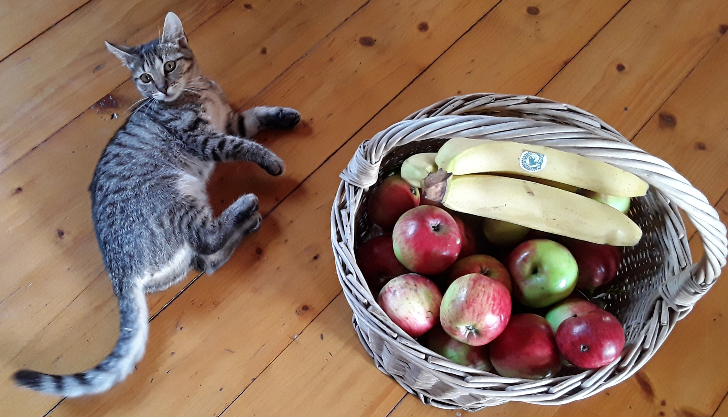
A - basket
B - fruits
Cat - noise
A - quantum computer
B - qubits
C - noise
What is a quantum computer?
Prodigious prospects of quantum computing
- Now: Not many distinct quantum algorithms
https://quantumalgorithmzoo.org/
Why?
- 00's Shor: Why have not more algorithms been found?
https://cs.brynmawr.edu/Courses/cs380/fall2012/Shor2003.pdf
Easy ones are efficient classically? We have no good language?

Click links at slides.com/marekgluza
- 90's Shor: quantum computers can break cryptography
- You could make money opening pandora boxes
- How long can you keep opening them? (Post-quantum cryptography)
Useful and important problems are not obviously efficiently solvable on a quantum computer...
What is a quantum computer?
A quantum computer is an experimental setup A which includes a quantum system B and that setup A allows to manipulate the quantum state of B.
Types of quantum computers:
- A) Superconducting loops
- B) Ionized atoms
- C) Neutral atoms
- D) Others
Companies:
- A) Google, IQM, IBM, Rigetti
- B) Quantinuum, IonQ
- C) Quera, Atom Computing, Pasqal
- D) Alice&Bob, Qolab, Normal Computing, Psi-Quantum,
Zapata
Currently 80 companies listed here:
https://thequantuminsider.com/2025/09/23/top-quantum-computing-companies/
Quantum computing cannot be useful if
- The problem can be solved quickly on classical computers
- Solving the problem isn't important
- Solving the problem is too hard for the quantum computer
Examples
- Trade bonding?
- Random sampling
- Mixed-integer programming? Shortest-vector problem? Etc.
Classical computation
Difficult, important and doable problem
Millenials
What challenge to take up?
What is a quantum computer made of?
A quantum computer is an experimental setup A which includes a quantum system B and that setup A allows to manipulate the quantum state of B.
Types of quantum computers:
- A) Superconducting loops
- B) Ionized atoms
- C) Neutral atoms
- D) Others
Advantages:
- A) Fabrication similar to Si pipelines
- B) Naturally quantum
- C) Large numbers
- D) Leverage pecularities
It is hard to do anything useful, now, without knowing the low-level physics of the devices: Think vacuum tubes rather than CMOS
Disadvantages:
- A) A-priori very noisy (but: arxiv:2408.13687)
- B) Scaling-up (but: arxiv:2511.05465)
- C) Unknown unknowns (arxiv:2412.15165)
- D) More risky (but: arxiv:abs/2307.06617)
Types of quantum computers:
- A) Superconducting loops
- B) Ionized atoms
- C) Neutral atoms
- D) Others
A quantum computer is an experimental setup A which includes a quantum system B and that setup A allows to manipulate the quantum state of B.
What is a quantum computer made of?
It is hard to do anything useful, now, without knowing the low-level physics of the devices: Think vacuum tubes rather than CMOS
What is a good quantum computer?
A quantum computer is an experimental setup A which includes a quantum system B and that setup A allows to manipulate the quantum state of B.
Outperforming your laptop:
- A) Superconducting loops (Google)
- B) Ionized atoms (Quantinuum)
- C) Neutral atoms (Quera)
Initially:
- What's the apriori quality of B?
- How do you make B modular?
- How good is setup A in manipulating B?
- What does A leverage against noise?


What is a powerful quantum computer?
A quantum computer is an experimental setup A which includes a quantum system B and that setup A allows to manipulate the quantum state of B.
Eventually:
- How much error-correction required?
- How many qubits can you cram?
- Speed of elementary gates?
- Overheads for real-world problems?
Utility-scale: When quantum computers will not be limited by noise in what they can do. We assume things will be just fine from then on! (?)

If you had a perfect quantum computer today - what would you use it for?
Outperforming your laptop:
- A) Superconducting loops (Google)
- B) Ionized atoms (Quantinuum)
- C) Neutral atoms (Quera)
What challenge to take up?
Materials science?
Quantum computing cannot be useful if
- The problem can be solved quickly on classical computers
- Solving the problem isn't important
- Solving the problem is too hard for the quantum computer
Examples
- Trade bonding?
- Random sampling
- Mixed-integer programming? Shortest-vector problem? Etc.
When a lot of people can gain by having something to say, some will not resist the temptation to speak without having much to tell which creates hype
Why materials science? Imagine improving photovoltaics by 1%.
What is needed? Prepare low-energy state of the material and study its physics.
How? Optimization quantum algorithms and physics research.
0
0
0
0
C
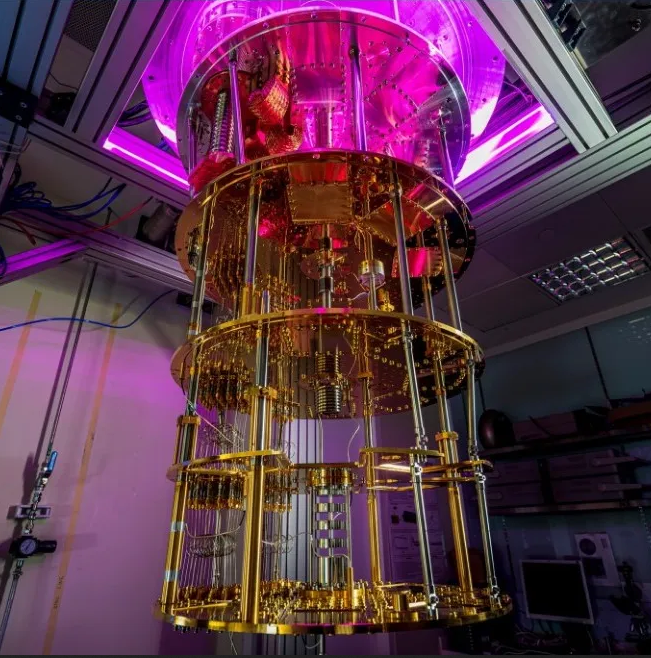
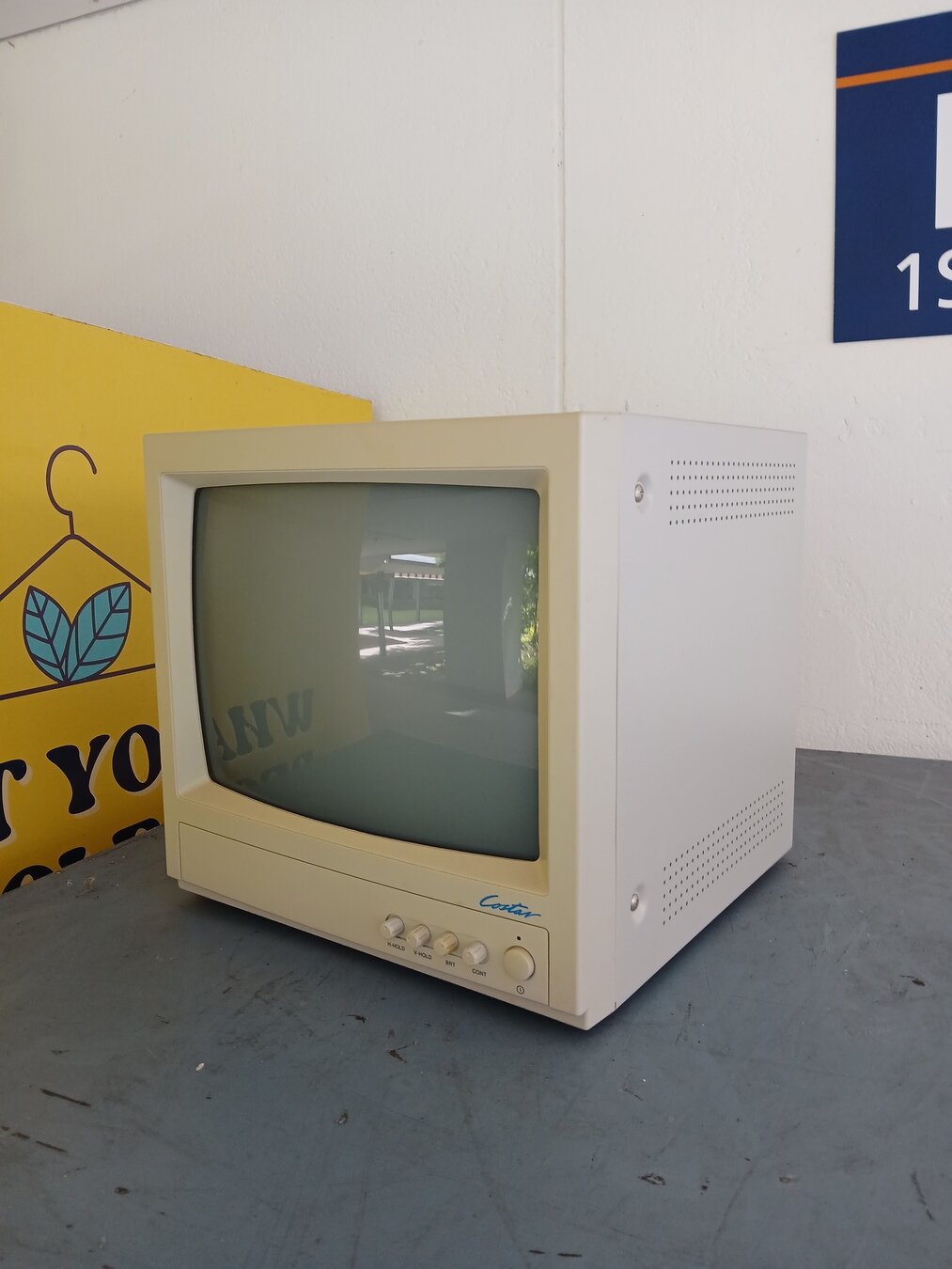
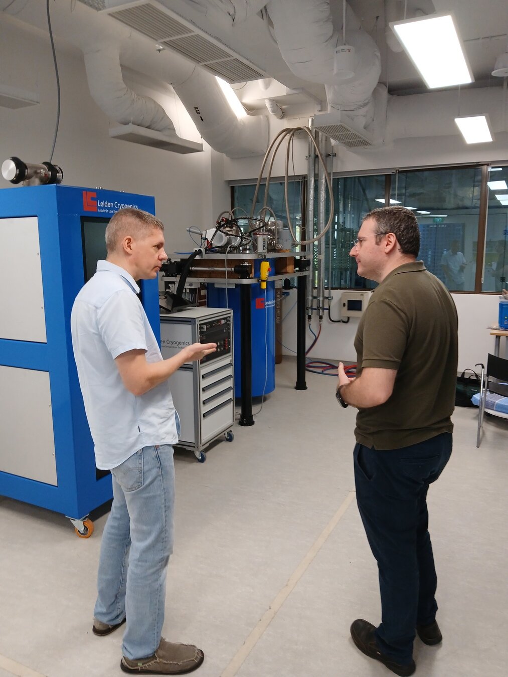
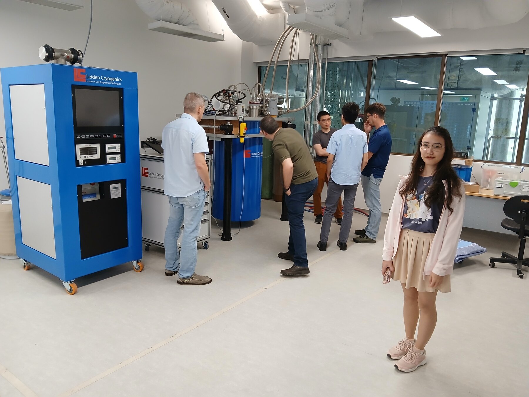
This monumental structure is the insides of the dilution refrigerator, shielding qubits from noise and guiding control lines inside.
A - basket
B - fruits
Cat - noise
A - quantum computer
B - qubits
C - noise
- Breaking RSA will be disruptive.
- Materials science could be constructive.
- Quantum computers efficiently simulate processes in nature and cooling of materials occurs in nature.
- The entire community searched for general optimization speed-ups but rests hope on heuristics.
What will quantum computer do?
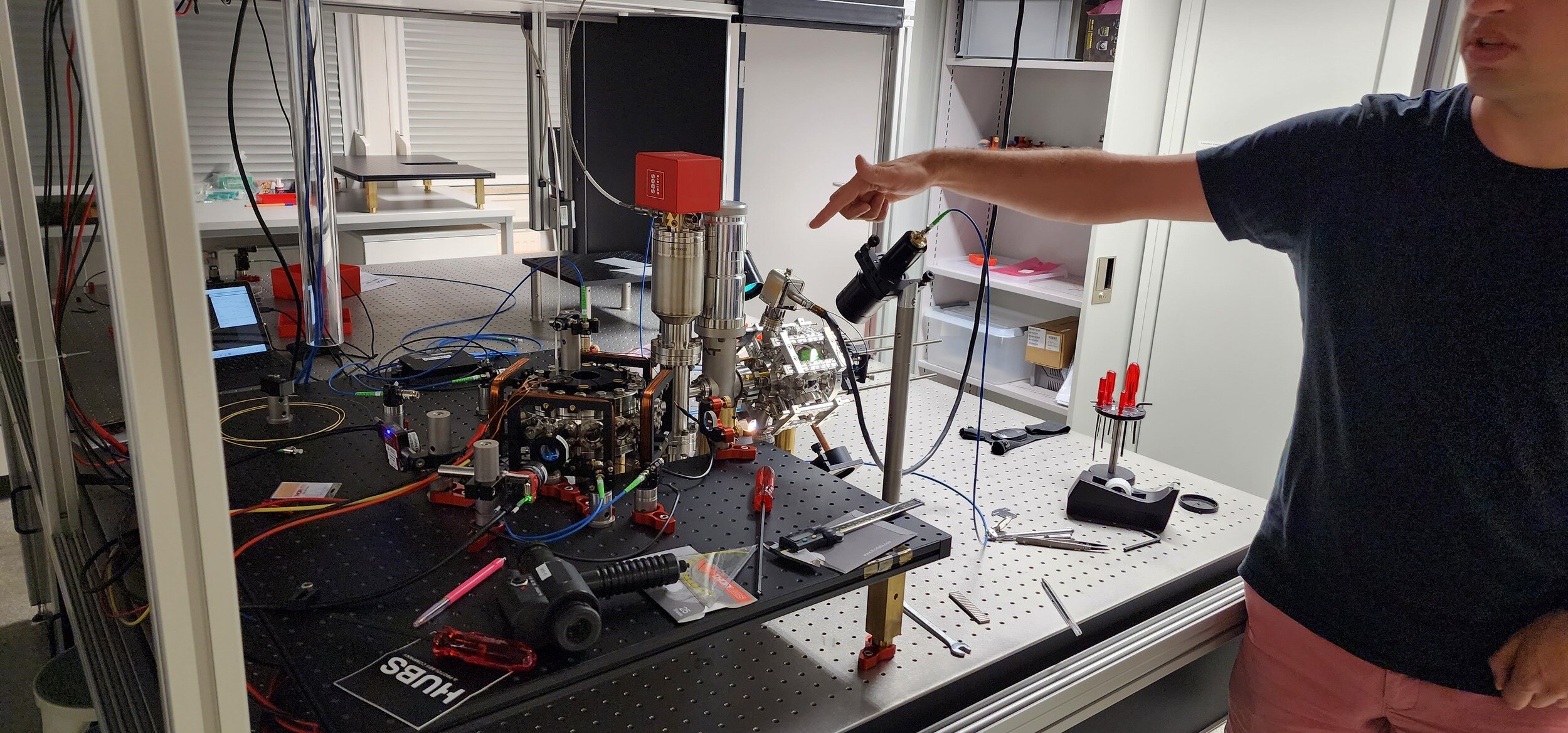
Symptomatic of detail complexity in quantum computing hardware: The 'casing' of the computer can be as important as the 'processor'.
Current phase: Break-even between wisdom and naivety.
0
0
0
0
C
A - quantum computer
B - qubits
C - noise
A quantum computer is an experimental setup A which includes a quantum system B and that setup A allows to manipulate the quantum state of B.
This is modeled by mulitplying unitary matrices to vectors from a finite-dimensional vector space.
What is the mathematical model?
Quantum system B is modeled by a finite dimensional vector space \(\mathcal V = \mathbb C^d\)
Having \(n\) qubits means tensor product structure \(\mathcal V = (\mathbb C^2)^{\otimes n}\) and \(d=2^n\)
Quantum gates are unitary matrices
Braket notation
1 qubit:
*The biography of the physicist who proposed it is literally called "The strangest man"

*Dirac was one of the smartest quantum physicist in history
"ket"
"bra"
"bracket"
"quantum superposition"
What is a universal quantum computer?
1 qubit
2 qubits
3 qubits
4 qubits
it can approximate any state preparation via circuits
It is a machine for realizing such linear combinations in nature
0
0
0
0
C
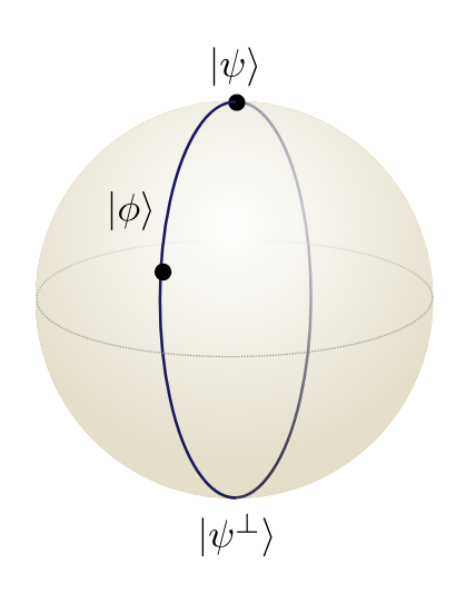
Operating a quantum computer is all about the group of unitary matrices
Think of rotations on a sphere
Operating a quantum computer is all about the group of unitary matrices
Think of rotations on a sphere
Universal quantum computation means: Composing sufficiently many basic unitary matrices (elementary quantum gates \(G_1,G_2,\ldots, G_K\)) can approximate any other 'larger' unitary.
(finding these sequences = task of unitary synthesis)
4 stages of creating quantum algorithms
1. Design choice:
How to go about it?
2. Unitary synthesis:
How to do it?

3. Circuit compilation:
What gates to do?
0. Problem choice:
What challenge to take up?
Double-bracket quantum algorithms:
Systematic framework for unitary synthesis
Riemannian geometry leads to quantum algorithms
Next: How to get $$ from a quantum computer?
We need to optimize among all operations of the quantum computer to get a low-energy state
(Riemannian optimization)
Marek Gluza
The double-bracket quantum algorithms roadmap
...the outline of the talk
Today, I will tell you about double-bracket quantum algorithms
Part 1: What is quantum computing?
Part 2: Riemannian geometry of the unitary group
Part 3: Optimization solvers from basic properties of the unitary group
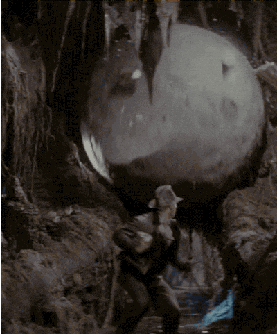
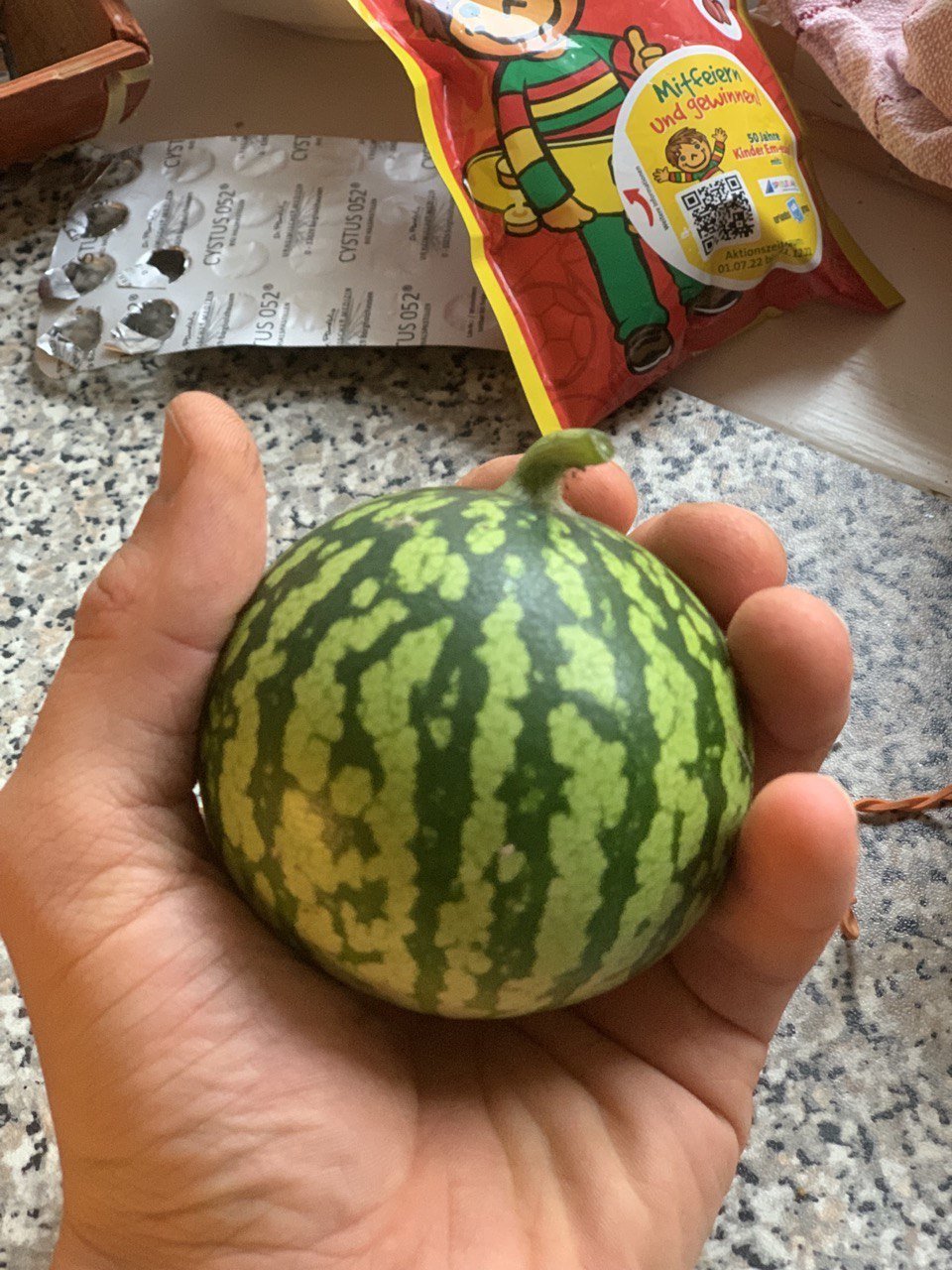
Next: Why a watermelon?
This visualizes the operations on a quantum computer
(Riemannian geometry)
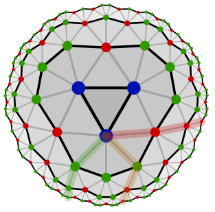
- Riemannian geometry is a generalization of the geometry of the sphere
- For 1 qubit the sphere is a great model of quantum operations
- In higher dimensions many parallels remain e.g. set of quantum operations is compact (the watermelon fits into the hand) but many get lost e.g. non-convex submanifolds (green colors on the watermelon)
- If watermelon is placed on the table then the table is tangent to it
This visualizes the operations on a quantum computer
(Riemannian geometry)
- Riemannian geometry is a generalization of the geometry of the sphere
- For 1 qubit the sphere is a great model of quantum operations
- In higher dimensions many parallels remain e.g. set of quantum operations is compact (the watermelon fits into the hand) but many get lost e.g. non-convex submanifolds (green colors on the watermelon)
- If watermelon is placed on the table then the table is tangent to it
Next: Let's see how to use geometry to design quantum algorithms
Riemannian geometry is essential for quantum computation
- The unitary group \(U(d)\) is a Riemannian manifold
- It is an embedded manifold \(U(d) = \{M\in \mathbb C^{d\times d}:~M^{-1}=M^\dagger\}\)
- The tangent space is \(\{W\in \mathbb C^{d\times d}:~W^{\dagger}= -W\} \simeq\{iH \mathrm{~where~} H=H^\dagger\in \mathbb C^{d\times d}\} \)
- The geodesics are matrix exponentials \( \{e^{sW}\}_{s\in\mathbb R} \subset U(d)\) or \( \{e^{isH}\}_{s\in\mathbb R} \subset U(d)\)
- Computing a "gradient" must output an element of the tangent space

\(\partial_{i,j}\) points to the interior, not tangential
Keep this in mind for later: Unlike in flat space, these 4 steps spiral away from the point of origin
Riemannian geometry is essential for quantum computation
- The unitary group \(U(d)\) is a Riemannian manifold
- The tangent space is \(\{H\in \mathbb C^{d\times d}:~H^{\dagger}= H\} \)
- The geodesics are matrix exponentials \( \{e^{isH}\}_{s\in\mathbb R} \subset U(d)\)
- \(U(d)\) is a curved manifold
Operating a quantum computer is all about the group of unitary matrices
Think of rotations on a sphere
The Lie bracket of two 'velocities' is again a velocity:
Check: \([A,B]^\dagger = (AB- BA)^\dagger = B^\dagger A^\dagger -A^\dagger B^\dagger = -[A,B]\)
\([A,B]^\dagger = -[A,B]\)
Check: \([A,B]^\dagger = -[A,B]\)
Operating a quantum computer is all about the group of unitary matrices
Think of rotations on a sphere
Fact 3: The Lie bracket of two 'velocities' is again a velocity
Operating a quantum computer is all about the group of unitary matrices
Think of rotations on a sphere
Fact 3: The Lie bracket of two 'velocities' is again a velocity
My quantum algorithms use such unitary matrices - they are implementing Riemannian gradient descent
The main tool of double-bracket quantum algorithms
Marek Gluza
The double-bracket quantum algorithms roadmap
...the outline of the talk
Today, I will tell you about double-bracket quantum algorithms
Part 1: What is quantum computing?
Part 2: Riemannian geometry of the unitary group
Part 3: Optimization solvers from basic properties of the unitary group
Note that choosing \(A=H\) doesn't change the energy
Let's find which directions \(A\) are more useful!
\(\partial_{i,j}\) points to the interior, not tangential so which direction is best?
Riemannian gradient: Unique vector \(g\) in the tangent space
such that the directional derivative is a projection onto \(g\)
\(\partial_{i,j}\) points to the interior, not tangential so which direction is best?
We will use very simple ingredients to find \(g\) for \(E(\psi) = \langle \psi| H | \psi\rangle\):
Hilbert-Schmidt scalar product:
Cyclicity of trace:
Tangent space:
Riemannian gradient: Unique vector \(g\) in the tangent space such that the directional derivative is a projection onto \(g\)
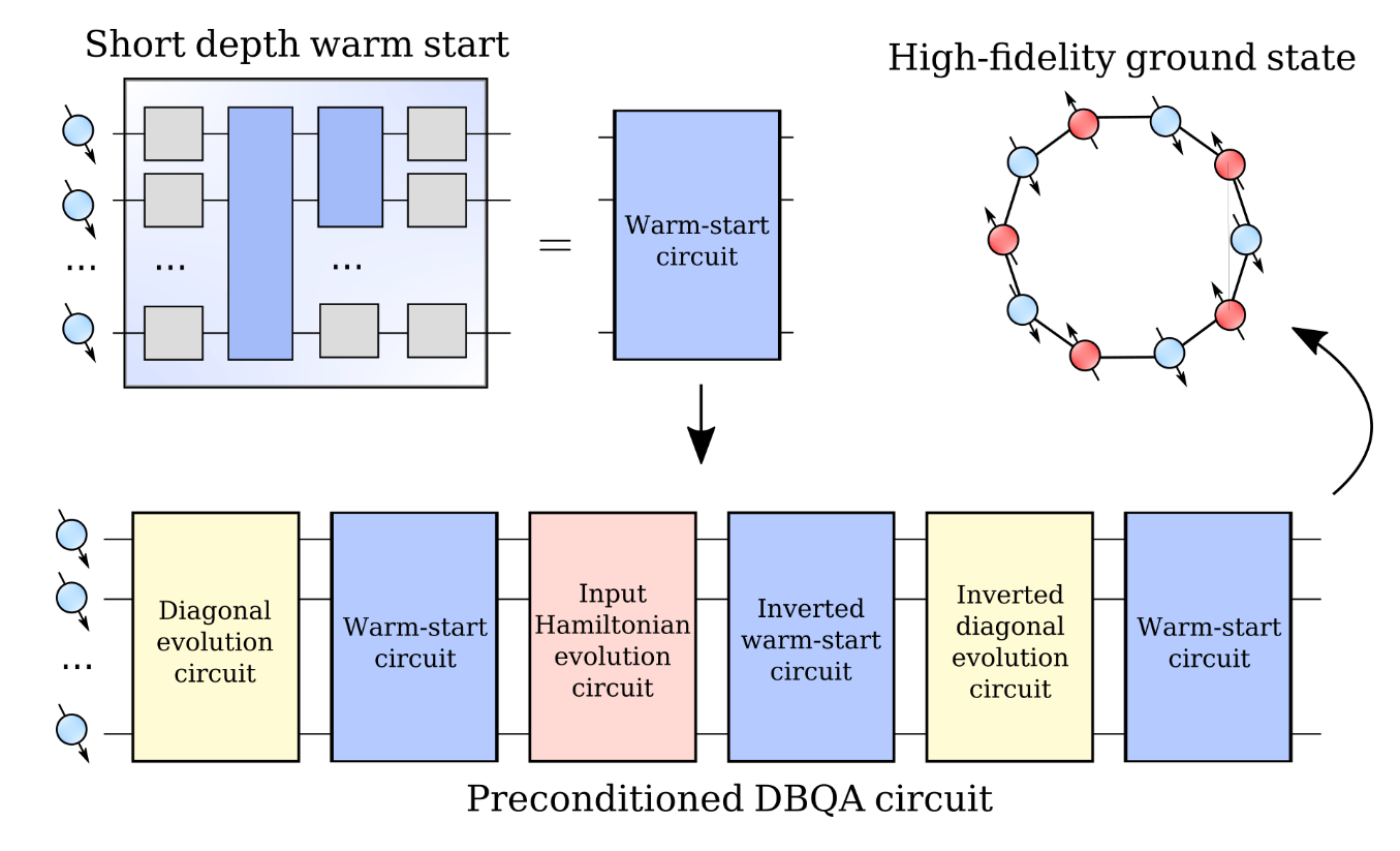
Double-bracket quantum algorithms:
Systematic framework for implementing exponentials of commutators on quantum computers. This uncovered new unitary synthesis formulas.
Riemannian gradient: Unique vector \(g\) in the tangent space such that the directional derivative is a projection onto \(g\)
Double-bracket flows
|
Heisenberg equation |
Linear, variable: observable |
|---|---|
|
Schroedinger equation |
Linear, variable: density matrix |
|
Double-bracket flow |
Non-linear, variable: density matrix or observable The solution is a unitary rotation because |
Why double a bracket?
2 qubit unitary
Canonical
Double-bracket quantum algorithms
are inspired by double-bracket flows
and allow to perform optimization through short quantum computations
Marek Gluza
The double-bracket quantum algorithms roadmap
...the outline of the talk
Today, I will tell you about double-bracket quantum algorithms
Part 1: What is quantum computing?
Part 2: Riemannian geometry of the unitary group
Part 3: Optimization solvers from basic properties of the unitary group

4 stages of creating quantum algorithms
1. Design choice:
How to go about it?
3. Circuit compilation:
What gates to do?
0. Problem choice:
What challenge to take up?
2. Unitary synthesis:
How to do it?
Double-bracket quantum algorithms:
Systematic framework for unitary synthesis
4 stages of creating quantum algorithms
Marek Gluza
The double-bracket quantum algorithms roadmap
I grew up around these mountains where Poland meets Czech Republic and Slovakia (in Europe)
June '22: Single-author double-bracket proposal

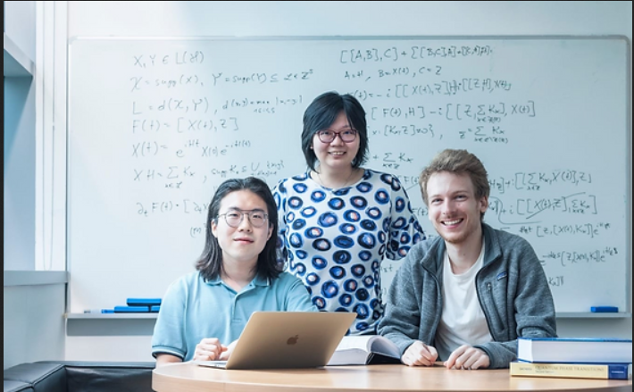
This talk is an overview of 4 years of my research on double-bracket quantum algorithms:
- Never worked on quantum algorithms before \(\rightarrow\) 9 papers, 1 experiment
- Never participated in a research program \(\rightarrow\) lead a collaboration of 25 co-authors
- It was the mathematical observations guiding us \(\rightarrow\) Riemannian geometry is key!
[1]
[9]
[8]
[5]
[2]
[3,4]
[6]
[7]
Click these links at slides.com/marekgluza

October '21: Arrived to Singapore
Double-bracket quantum algorithms
Click these links at slides.com/marekgluza
| Diagonalization | https://arxiv.org/abs/2206.11772 | ||
|---|---|---|---|
| Imaginary-time evolution | https://arxiv.org/abs/2412.04554 | ||
| Quantum signal processing | https://arxiv.org/abs/2504.01077 | ||
| Grover's search | https://arxiv.org/abs/2507.15065 | Approximates ITE |
Solve the unitary synthesis problem in all these cases through Riemannian gradients!
4 stages of creating quantum algorithms
1. Design choice:
How to go about it?
3. Circuit compilation:
What gates to do?
0. Problem choice:
What challenge to take up?
2. Unitary synthesis:
How to do it?
4 stages of creating quantum algorithms
Imaginary-time evolution
4 stages of creating quantum algorithms
1. Design choice:
How to go about it?
3. Circuit compilation:
What gates to do?
0. Problem choice:
What challenge to take up?
2. Unitary synthesis:
How to do it?
4 stages of creating quantum algorithms
Breather pause for time check. Next either:
A) 2 mins and 42 seconds to complete the process of unitary synthesis
B) or wrap up?
4 stages of creating quantum algorithms
1. Design choice:
How to go about it?
3. Circuit compilation:
What gates to do?
0. Problem choice:
What challenge to take up?
2. Unitary synthesis:
How to do it?
4 stages of creating quantum algorithms
4 stages of creating quantum algorithms
4 stages of creating quantum algorithms
2. Unitary synthesis:
How to do it?
1. Design choice:
How to go about it?
3. Circuit compilation:
What gates to do?
0. Problem choice:
What challenge to take up?
Product formula approximation:
\(e^{\tau[|\psi\rangle\langle\psi|,H]}| = e^{i\sqrt{\tau}H}e^{i\sqrt{\tau}|\psi\rangle\langle\psi|}e^{-i\sqrt{\tau}H}e^{-i\sqrt{\tau}|\psi\rangle\langle\psi|} + O(\tau^{3/2})\)
Product formula approximation:
\(e^{\tau[|\psi\rangle\langle\psi|,H]}| = e^{i\sqrt{\tau}H}e^{i\sqrt{\tau}|\psi\rangle\langle\psi|}e^{-i\sqrt{\tau}H}e^{-i\sqrt{\tau}|\psi\rangle\langle\psi|} + O(\tau^{3/2})\)
Quantum algorithm DB-QITE - iterate recursively:
- Define \(|{\psi_k}\rangle = U_k |0\rangle\)
- Use \(e^{is |\psi_k\rangle\langle\psi_k|} = U_ke^{is |0\rangle\langle0|}U_k^\dagger \)
- Recursively iterate \( U_{k+1} = e^{is H} U_k e^{is |0\rangle\langle 0|} U_k^\dagger e^{-is H} U_k\)
3 stages of creating quantum algorithms
1. Design choice:
How to go about it?
3. Circuit compilation:
What gates to do?
0. Problem choice:
What challenge to take up?
4 stages of creating quantum algorithms
2. Unitary synthesis:
How to do it?

(accepted at PRL)
Product formula approximation:
\(e^{\tau[|\psi\rangle\langle\psi|,H]}| = e^{i\sqrt{\tau}H}e^{i\sqrt{\tau}|\psi\rangle\langle\psi|}e^{-i\sqrt{\tau}H}e^{-i\sqrt{\tau}|\psi\rangle\langle\psi|} + O(\tau^{3/2})\)
Quantum algorithm DB-QITE - iterate recursively:
- Define \(|{\psi_k}\rangle = U_k |0\rangle\)
- Use \(e^{is |\psi_k\rangle\langle\psi_k|} = U_ke^{is |0\rangle\langle0|}U_k^\dagger \)
- Recursively iterate \( U_{k+1} = e^{is H} U_k e^{is |0\rangle\langle 0|} U_k^\dagger e^{-is H} U_k\)
3 stages of creating quantum algorithms
1. Design choice:
How to go about it?
3. Circuit compilation:
What gates to do?
0. Problem choice:
What challenge to take up?
4 stages of creating quantum algorithms
2. Unitary synthesis:
How to do it?
(accepted at PRL)
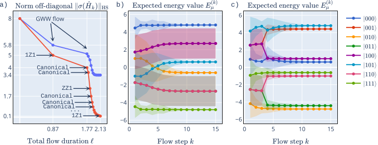
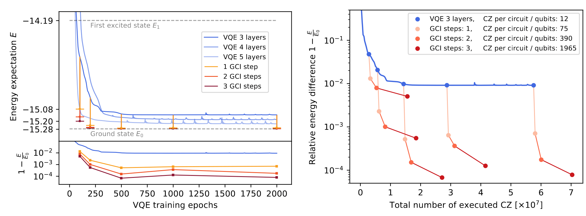
Numerical results for DB-QITE:
DB-QITE:
- Define \(|{\psi_k}\rangle = U_k |0\rangle\)
- Recursively iterate \( U_{k+1} = e^{is H} U_k e^{is |0\rangle\langle 0|} U_k^\dagger e^{-is H} U_k\)
Then:


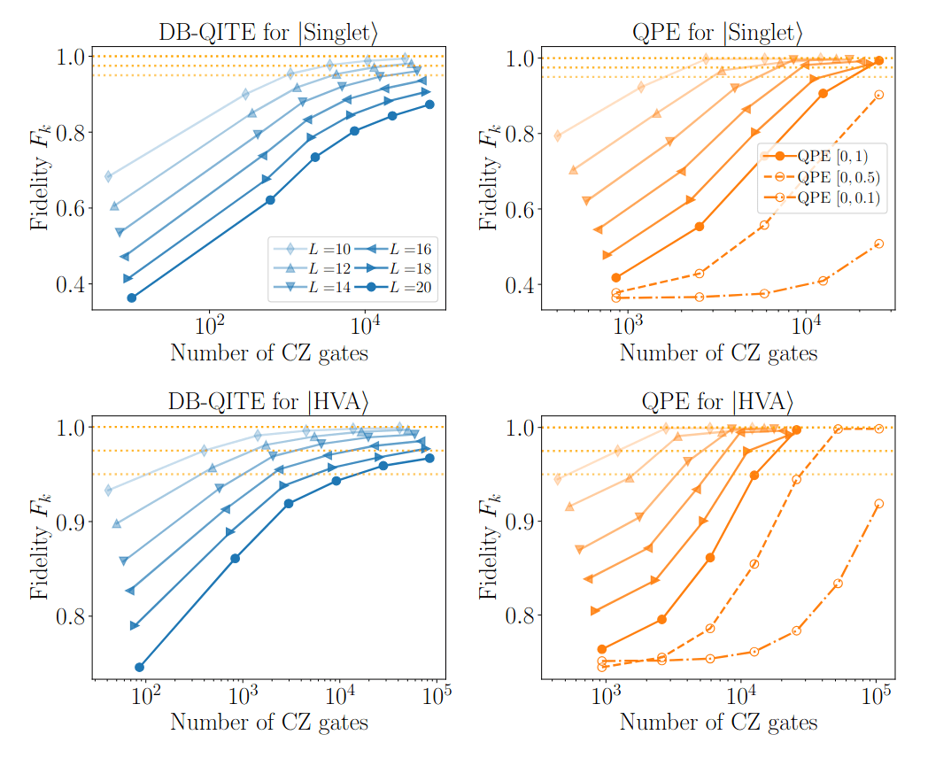
Quantinuum
(accepted at PRL)
Double-bracket quantum algorithms
- Coherently implement Riemannian gradient steps
-
Give rigorous unitary synthesis for
- imaginary-time evolution
- quantum signal processing
- diagonalization unitaries
- Grover's as an approximation to imaginary-time evolution
- Training quantum circuits from data doesn't work well, unlike in classical machine learning applications. However those variational learning methods are great for warm-starting double-bracket quantum algorithms!
Tell me when not fast enough? Get stuck? Something else?
Your input is needed to improve them!
N. Ng
Z. Holmes
R. Zander
R. Seidel

Y. Suzuki
B. Tiang
J. Son
S. Carrazza
Stay in touch on LinkedIn:
Text
Text
Text
Marek Gluza
Quantum algorithmic control of quantum systems
Arrived to Singpore in 2021
[7,9,12,13]
PRL, Scipost x2, Nature Physics

[4] PRL

[5,10,14,19,24]
PNAS, PRL, CP,...
[8] PNAS
[16,17,23]


[15,21,25]
[11,18,20]
[22]
[6]


Large numerical simulations
Tensor-network simulations
Theory for quantum fields
Material science key application of quantum simulation?
Protocol independently used by Google
Computer science result for physics
Material science?
Experimental protocols
J. Schmiedmayer
Mathematical physics
J. Eisert
Large numerical simulations
Tensor-network simulations
Theory for quantum fields
Material science key application of quantum simulation?
Fidelity witness protocol independently used by Google AI
Computer science result for physics
Experimental protocols
J. Schmiedmayer
Mathematical physics
J. Eisert
Goals?
Realistic?
Intuition?
Quantum computer
Quantum algorithm
Cooling
Natural
0
0
0
0
C
[1] Double-bracket quantum algorithms for diagonalization
YES!!!!
Singapore's
quantum computer
R. Dumke
S. Carrazza

Optimizing a random guess to cool gets stuck
Can't do material science?! :(
DBQA moves it ahead!
[3]
We know how to make it run fast!
Quantum gates
N. Ng
Exactly how good is it?
[2]
Singapore's
quantum computer
R. Dumke
S. Carrazza
R. Takagi
N. Ng
0
0
0
0
C
[1] Double-bracket quantum algorithms for diagonalization
Z. Holmes
S. Carrazza
[3] Double-bracket quantum algorithms for high-fidelity ground state preparation
[2]
Quantum algorithmic control of quantum systems
Demonstrate tangible advantages
from quantum computing
Phase 1
Phase 2
Collaboration with industry: need best available hardware
Demonstrate that DBQA
enable advances in material science
WP1: Programming natural
quantum systems
Physics output
Quantum dynamic programming
on SG QPUs
Deliver Qibo
software for NQCH demonstrations
WP2: Programming Singapore's
QPUs
Software output
Tame physics obstructions to running long quantum computations
Deliver systematic and automated calibration routines for SG QPUs

Expand quantum algorithmic insights beyond quantum computing
Enhance spectroscopy of molecules

Apply accross industry and academia
Deliver Qibo drivers & quantum arcade
New SG export area: Quantum algorithms
SG network with leading quantum computing companies in the US and EU
Aim: 23 publications, 1 quantum arcade
Team in place: 2x RA, 2x FYP, network
Motto: Each interaction with a team member shall make them stronger
Regular expertise tutorials
Professional Qibo software development
Notion timelines
Key collaborators:
- S. Carrazza, N. Ng, Z. Holmes, K. Mitarai, M. Murao, J. Knoerzer, L. Aolita, T.-S. Koh, I. Marvian, P. Kos, M. Huber, + P. Zoller & J. Eisert ...
- R. Dumke, J.-Y. Khoo, S.-T. Goh, L. Yang, D. Campolo, K. Bharti, ...
4 stages of creating quantum algorithms
1. Design choice:
How to go about it?
2. Unitary synthesis:
How to do it?
3. Circuit compilation:
What gates to do?
0. Problem choice:
What challenge to take up?
Double-bracket quantum algorithms:
Systematic framework for unitary synthesis
4 stages of creating quantum algorithms
How to go about designing quantum algorithms?
- Now: Not many distinct quantum algorithms
https://quantumalgorithmzoo.org/ - Why?
- Classically: Reduction to decision problems
- Quantumly: Is \(\langle\psi|H|\psi\rangle\) lower than ...?
- Optimization: Only quadratic speed-up?
- "Grand unification of quantum algorithms" https://arxiv.org/abs/2105.02859 the block-encoding scheme for accessing \(H\)
- This talk: Another unification based on Riemannian optimization and using geodesics \(e^{isH}\) to access \(H\)
- Double-bracket quantum algorithms give intuition why unification possible: \(\langle\psi|H|\psi\rangle\) is optimization so interpret through Riemannian gradients
Click links at slides.com/marekgluza
What is quantum signal processing?
Example 1: Exponential function
Example 2: Polynomial approximation to exponential
Example 3: Polynomial approximation to inversion
Quantum signal processing maps between states according to a polynomial filter
Approach 2. Exponentials of commutators
- Recursive ~ exponentially long circuits
- Double-bracket quantum algorithms link to Riemannian gradients
Approach 1. Block-encodings
- Probablistic ~ exponentially unlikely postselection
- Grand unification of quantum algorithms https://arxiv.org/abs/2105.02859