Sums and infinite sums

S_2 = 1 + 1/2 = 1.5

S_3 = 1 + 1/2 + 1/4 = 1.75

S_4 = 1 + 1/2 + 1/4 +1/8 = 1.875

In times of Euler, mathematics was an experimental science:

What will be the value of \(S_\infty\)?

S_\infty = 1 + 1/2 + 1/4 +1/8 + \ldots

Will it exceed \(S_\infty>2\)?

Sums and infinite sums

Let us use a trick:

Euler (and later Ramanujan) was famous for playing with infinite sums. This trick works but Euler made mistakes too. Generations of mathematicians after him had to provide a proof that his intuition was correct.

S_\infty = 1 + 1/2\times (1+1/2 + 1/4 + \ldots )

S_\infty = 1 + 1/2 \times S _\infty

1/2 \times S_\infty = 1

S_\infty = 2

Sums and infinite sums

S_\infty = 1 + 1/2+ 1/4 + \ldots \\

S_\infty(q) = \lim_{N\rightarrow\infty}\sum_{n=0}^N q^n = \lim_{N\rightarrow \infty} \frac{1-q^{N+1}}{1-q}

S_\infty(q) = \sum_{n=0}^\infty q^n = \frac{1}{1-q} \quad\text{if}\quad |q|< 1

Check: \(S_\infty(q=1/2) = 1 / (1-1/2) =2\)

The exponential function

\quad\text{where}\quad n! = 1\cdot 2\cdot 3\cdot\ldots \cdot n

e^x = \sum_{n=0}^\infty \frac{1}{n!} x^n

x\in\mathbb R

Above, \(|q|<1\) was a restriction. Here \(1/n!\) coefficients remove the restriction and \(x\in \mathbb R\) can be arbitrary.

S_\infty(q) = \sum_{n=0}^\infty q^n = \frac{1}{1-q} \quad\text{if}\quad |q|< 1

We understood \(q\in \mathbb C\). What if \(q\) was a matrix?

Check: It makes sense to ask this because if \(A\in \mathbb C ^{d\times d} \) then \(A^k\in \mathbb C ^{d\times d} \) and we can add matrices of the same dimension.

S_\infty(A) = \sum_{n=0}^\infty A^n = \frac{I}{I-A} \quad\text{if}\quad \max_{i,j}|A_{i,j}|< 1/d

Quantum mechanics

used to be called matrix mechanics

Matrix inversion?!

Quantum mechanics

is all about exponentials

If \(A\in \mathbb C ^{n\times n} \) then we can define the exponential:

e^A = \sum_{n=0}^\infty \frac{1}{n!} A^n

It means: multiply the matrix with itself \(n\) times and sum it up with the coefficient \(1/n!\)

I cannot draw a picture of \(e^A\) like for \(e^x\). But I will show you why choosing \(A\) to be \(A = \begin{pmatrix} 0 &1\\-1 & 0\end{pmatrix}\) is useful in quantum computing.

\sum_{n=0}^\infty A^n = \frac{I}{I-A}

\text{if}\quad \max_{i,j}|A_{i,j}|< 1/d

It means: multiply the matrix with itself \(n\) times and sum it up with the coefficient \(1/n!\) (this was missing before).

Outline:

Infinite sums
Euler's formula
Infinite products

Euler was studying complex numbers:

\(z = x+iy\) where \(x,y\in \mathbb R\) and \(i^2 = -1\)

He asked: What would be the exponential of a purely complex number \(e^{z} = e^{iy}\)?

e^z = \sum_{n=0}^\infty \frac{1}{n!} z^n

= 1 + i y + \frac 12 i^2 y^2 + \frac 1 6i^3 y^3 + \ldots

= 1 + i y -\frac 12 y^2 - \frac 1 6i y^3 + \ldots

Euler wrote 800 manuscripts in his life, they included many formulas.

But what he found here is usually called the Euler's formula.

Euler was studying complex numbers:

\(z = x+iy\) where \(x,y\in \mathbb R\) and \(i^2 = -1\)

He asked: What would be the exponential of a purely complex number \(e^{z} = e^{iy}\)?

\sin(x) = \sum_{n=0}^\infty (-1)^n \frac{x^{2n+1} }{(2n+1)! } = x-\frac 16x^3+ \ldots

\cos(x) = \sum_{n=0}^\infty (-1)^n \frac{x^{2n} }{(2n)! } = 1-\frac 12 x^2+ \ldots

e^z = \sum_{n=0}^\infty \frac{1}{n!} z^n

= 1 + i y + \frac 12 i^2 y^2 + \frac 1 6i^3 y^3 + \ldots

= 1 + i y -\frac 12 y^2 - \frac 1 6i y^3 + \ldots

e^{iy} =\cos(y) + i \sin(y)

Braket notation

\mathcal V = \mathbb C^2 = \mathrm{span}_{\mathbb C}\{ e_1, e_2\}

| 0 \rangle :=e_1, | 1\rangle :=e_2

\vec v \in \mathcal V \leftrightarrow |v\rangle = v_0 | 0 \rangle + v_1 | 1\rangle

U \vec v \leftrightarrow U|\psi\rangle

"ket"

"quantum superposition"

In quantum computing, the state of a single qubit is a 2-dimensional vector \(\ket\psi = a \ket{0} +b\ket{1}\).

An operation with duration \(t\) and generated by \(Y=Y^\dagger \in\mathbb{C}^{2\times 2}\) is given by

Quantum computing operation a qubit is given by multiplying a 2-dimensional matrix to that vector.

U = e^{it Y} = \sum_{n=0}^\infty \frac 1{n!} (it)^n Y^n

"quantum evolution"

How can we create \( \frac1 {\sqrt 2} \ket{0} +\frac 1 {\sqrt 2}\ket{1}\)?

e^{i t Y }= \sum_{n=0}^\infty \frac{1}{n!} (i t)^n Y^n

= I + it Y + \frac 12 i^2 t^2 Y^2 + \frac 1 6i^3 t^3 Y^3 + \ldots

= I + i tY-\frac 12 t^2 Y^2 - \frac 1 6i t^3 Y^3 + \ldots

It has the properties

\(Y^2 = I\) and \(Y\ket 0 = - i \ket 1\)

Let us study the matrix \(Y = \begin{pmatrix} 0 &-i\\i & 0\end{pmatrix}\)

It can be engineered by applying oscillatory electromagnetic fields to the qubit.

= I + i tY-\frac 12 t^2 I - \frac 1 6i t^3 Y + \ldots

e^{itY} =\cos(t)I + i \sin(t) Y

e^{itY} \ket 0 =\cos(t)\ket 0 + i \sin(t) Y\ket 0 = \cos(t)\ket 0 + i \sin(t)(-i)\ket 1

This is how we can 'program' the state of the qubit!

e^{it Y} \ket 0 =\cos(t) \ket 0 + \sin(t) \ket 1

Using Euler's formula to 'program a qubit

Outline:

Infinite sums
Euler's formula
Infinite products

Definition of the Euler number:

e =\lim_{N\rightarrow \infty} \left (1+\frac{1} N \right)^N

e^x = \lim_{N\rightarrow \infty} \left (1+\frac{x} N \right)^N

Example:

\(x = 2, N = 100 \)

e^2\approx \left (1+\frac{2} {100} \right)^{100}

e^2\approx 1.02 \times 1.02 \times \ldots 1.02

To think that you multiply the number \(1.02\) with itself \(100\) times and you will get an approximation of \(e^2 \approx 7.39\) - that's what people admire about Euler's formulas!

Infinite products

Definition of the Euler number:

e =\lim_{N\rightarrow \infty} \left (1+\frac{1} N \right)^N

e^x = \lim_{N\rightarrow \infty} \left (1+\frac{x} N \right)^N

e^{it Y} \ket 0 =\cos(t) \ket 0 + \sin(t) \ket 1

We saw that EM drive creates qubit oscillation:

What if we would remove the imaginary number \(i\)?

e^{t Y} \ket 0 =?

It is very difficult to implement it on a quantum computer but if we would find a way then we could make a lot of money solving problems in industry.

\lim_{t\rightarrow \infty} e^{t Y} \approx (I+tY /N)^N

The right-hand side is a polynomial and the protocol called quantum signal processing can be used to implement it on a quantum computer.

Ongoing research on quantum algorithms!

Definition of the Euler number:

e =\lim_{N\rightarrow \infty} \left (1+\frac{1} N \right)^N

e^x = \lim_{N\rightarrow \infty} \left (1+\frac{x} N \right)^N

e^{it Y} \ket 0 =\cos(t) \ket 0 + \sin(t) \ket 1

We saw that EM drive creates qubit oscillation:

What if we would remove the imaginary number i?

e^{t Y} \ket 0 =?

\lim_{t\rightarrow \infty} e^{t Y} \approx (1+tY /N)^N

The right-hand side is a polynomial and the protocol called quantum signal processing can be used to implement it on a quantum computer.

Ongoing research on quantum algorithms!

I'm not sure if Euler had ideas about quantum computations.

I am sure that if he was alive today then he would be working on quantum computing!

It is very difficult to implement it on a quantum computer but if we would find a way then we could make a lot of money solving problems in industry.

Double-bracket quantum algorithms for diagonalization

Marek Gluza

NTU Singapore

slides.com/marekgluza

https://arxiv.org/abs/2206.11772

Gate count after VQE warm-start:

https://arxiv.org/abs/2408.03987

C(z,z',t) \approx \frac{\langle \Delta\hat\varphi(z,t)\Delta\hat\varphi(z',t)\rangle}{ \Delta z^2 }

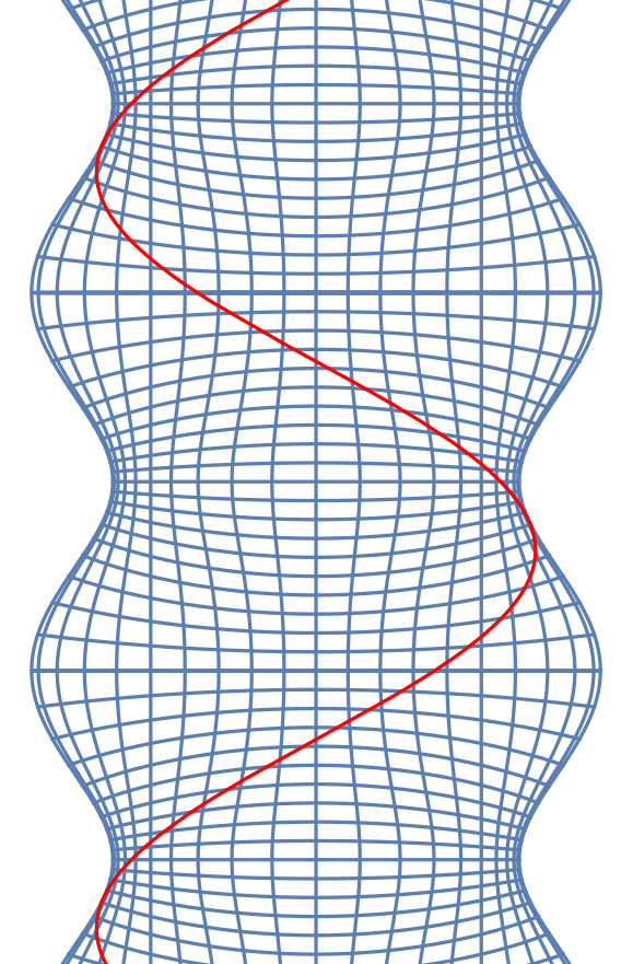
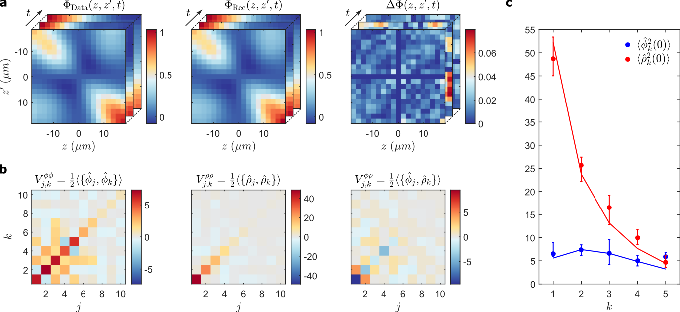
Experimental Observation of Curved Light-Cones in a Quantum Field Simulator

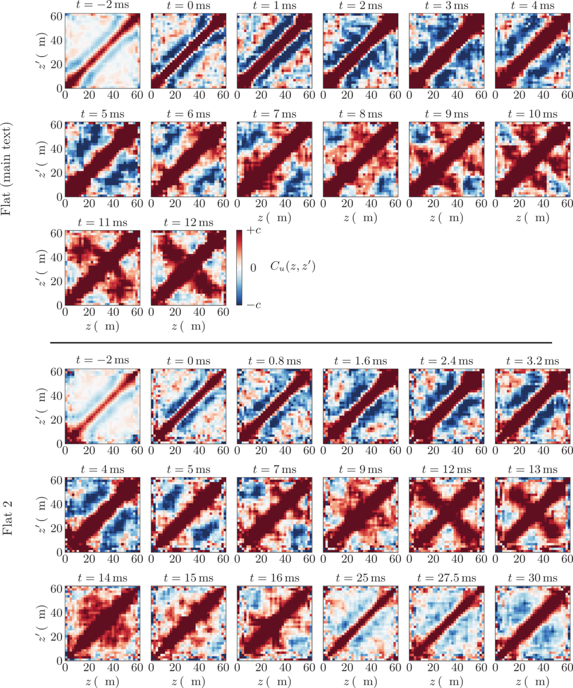
M. Tajik, J. Schmiedmayer

https://arxiv.org/abs/2209.09132

Breaking of Huygens-Fresnel principle in inhomogeneous Tomonaga-Luttinger liquids

Spyros Sotiriadis

https://arxiv.org/abs/2104.07751

Per Moosavi

\partial_{t}^{2} \hat{\phi} = 2 v(x) v'(x) \partial_{x} \hat{\phi} + v(x)^2 \partial^2_{x} \hat{\phi}

\partial_{t}^{2} \hat{\phi} = v(x)v'(x) \partial_{x} \hat{\phi} + v(x)^2\partial^2_{x} \hat{\phi}

\mapsto

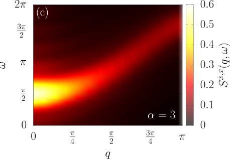
Tomography for phonons

\hat H_\text{TLL} = \int \text{d}z\left[ \frac{\hbar^2n_{GP}}{2m}\partial_z\hat\varphi^2+g\delta\hat\varrho^2\right]

\hat H_\text{TLL} = \sum_{k>0} \frac {\hbar \omega_k}2 (\phi_k^2+\delta\hat\rho_k^2) + g\rho_0^2

\langle\hat \phi_k^2(t)\rangle= \cos^2(\omega_k t) \langle \phi_k^2(0)\rangle \\ \quad\quad\quad\quad\quad+\sin^2(\omega_k t) \langle \delta\hat \rho_k^2(0)\rangle

\delta \hat\rho

\langle\hat \phi^2(t)\rangle

\langle\delta\hat \rho^2(0)\rangle =0?

\langle \hat \phi^2(0)\rangle

\hat \phi

https://arxiv.org/abs/1807.04567

https://arxiv.org/abs/2005.09000

Quantum mechanics

used to be called matrix mechanics

S_\infty(q) = \sum_{n=0}^\infty q^k = \frac{1}{1-q} \quad\text{if}\quad |q|< 1

We understood \(q\in \mathbb C\). What if \(q\) was a matrix?

Check: It makes because if \(A\in \mathbb C ^{n\times n} \) then \(A^k\in \mathbb C ^{n\times n} \) and we can add matrices of the same dimension.

S_\infty(A) = \sum_{n=0}^\infty A^k = \frac{1}{1-A} \quad\text{if}\quad \max_{i,j}|A_{i,j}|< 1

Examples of infinite sums

e^x = \sum_{n=0}^\infty \frac{1}{n!} x^k \quad\text{where}\quad n! = 1\cdot 2\cdot 3\cdot\ldots \cdot n

\sin(x) = \sum_{n=0}^\infty (-1)^k \frac{x^{2k+1} }{(2k+1)! } = x-\frac 13 x^3+ \ldots

\cos(x) = \sum_{n=0}^\infty (-1)^k \frac{x^{2k} }{(2k)! } = 1-\frac 12 x^2+ \ldots

Quantum mechanics

used to be called matrix mechanics

exp(A) = \sum_{n=0}^\infty \frac{1}{k!} A^k \quad\text{if}\quad \|A\| < ...?

\| \sum_{n=0}^N \frac{1}{k!} A^k \| \le \sum_{n=0}^N \frac{1}{k!} \|A^k \| \le exp(\|A\|)

\|exp(A)\| = \lim_{N\rightarrow \infty}\| \sum_{n=0}^N \frac{1}{k!} A^k \| \le exp(\|A\|)

\|A\| \ge 0

\|A+B\|\le \|A\| +\|B\|

\|\alpha A\|= |\alpha|\cdot \|A\|

\|A^k\|= \|A\|^k

Quantum mechanics

used to be called matrix mechanics

exp(A) = \sum_{n=0}^\infty \frac{1}{k!} A^k \quad\text{if}\quad \|A\| < ...?

S_\infty(A) = \sum_{n=0}^\infty A^k = \frac{1}{1-A} \quad\text{if}\quad \|A\|< 1

\| \sum_{n=0}^N \frac{1}{k!} A^k \| \le \sum_{n=0}^N \frac{1}{k!} \|A^k \| \le exp(\|A\|)

Why double a bracket?

\partial_t \hat A(t) = i [ \hat A(t), \hat H(t)]

\partial_t \hat A(t) = [ \hat A(t), [\hat A(t), \hat H(t)]]

Why double a bracket?

\partial_t \hat A(t) = i [ \hat H(t), \hat A(t)]

\partial_t \hat A(t) = [ \hat H(t), [\hat H(t), \hat A(t)]]

=

2 qubit unitary

Canonical

\partial_t \hat A(t) = [ \hat A(t), [\hat A(t), \hat H(t)]]

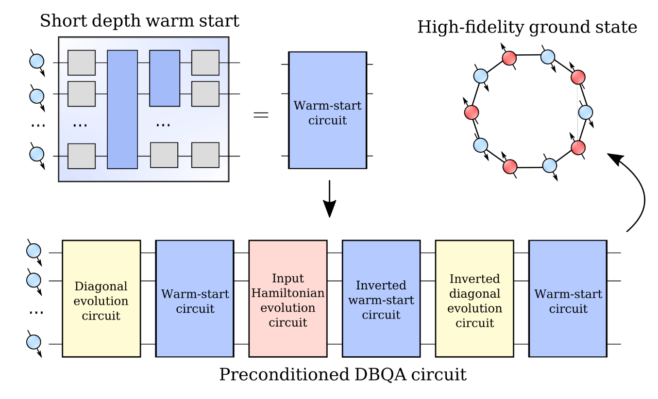
Double-bracket quantum algorithms

are inspired by double-bracket flows

and allow for quantum compiling of short-depth circuits which approximate grounds states

Inspired by double-bracket flows we compiled quantum circuits which yield quantum states relevant for material science

\partial_t \hat A(t) = [ \hat A(t), [\hat A(t), \hat H(t)]]

https://arxiv.org/abs/2408.03987

=

2 qubit unitary

Canonical

\hat H_1 = e^{s_0 \hat W_0} \hat H_0 e^{-s_0 \hat W_0}

\hat W_0 = [\hat D_0,\hat H_0]

Double-bracket rotation ansatz

antihermitian

\left(i\hat H\right)^\dagger = -i \hat H

Rotation generator:

Input:

Unitary rotation:

e^{s \hat W_0}

\hat H_0

Double-bracket rotation:

\partial_s \hat H_0(s) = [\hat W_0, \hat H_0]

\Leftrightarrow

\partial_s \hat H_0(s) = [\hat H_0(s),[ \hat H_0(0),\hat D_0] ]

\partial_t \hat A(t) = [ \hat A(t), [\hat A(t), \hat H(t)]]

\hat H_1 = e^{s_0 \hat W_0} \hat H_0 e^{-s_0 \hat W_0}

\hat W_0 = [\hat D_0,\hat H_0]

Double-bracket rotation ansatz

Rotation generator:

Input:

Unitary rotation:

e^{s \hat W_0}

\hat H_0

Double-bracket rotation:

Key point: If \(\hat D_0\) is diagonal then

\(\hat H_1\) should be "more" diagonal than \(\hat H_0\)

\hat H_0(s) = e^{s \hat W_0} \hat H_0 e^{-s \hat W_0}

\hat W_0 = [\hat D_0,\hat H_0]

Double-bracket rotation ansatz

Rotation generator:

Input:

\hat H_0

Double-bracket rotation:

\sigma(\hat H_0(s))

Restriction to off-diagonal

\partial_s \|\sigma(\hat H_0(s))\|_{\text{HS}}^2 = -2\langle \hat W_0,[\hat H_0, \sigma(\hat H_0)]\rangle_{\text{HS}}

Lemma:

Proof: Taylor expand, shuffle around (fun!)

\hat H(s) = e^{s \hat W_0} \hat H_0 e^{-s \hat W_0}

\hat W_0 = [\hat D_0,\hat H_0]

Double-bracket rotation ansatz

Rotation generator:

Input:

\hat H_0

Double-bracket rotation:

\sigma(\hat H_\ell)

Restriction to off-diagonal

\partial_s \|\sigma(\hat H_0(s))\|_{\text{HS}}^2 = -2\langle \hat W_0,[\hat H_0, \sigma(\hat H_0)]\rangle_{\text{HS}}

Lemma:

Proof: Taylor expand, shuffle around (fun!)

A new approach to diagonalization on a quantum computer

\hat H_1 = e^{s \hat W_1} \hat H e^{-s \hat W_1}

\hat W_k = [D_{k-1},\hat H_{k-1}]

\hat H_k = e^{s \hat W_k} \hat H_{k-1} e^{-s \hat W_k}

\hat H_\text{TFIM} = \sum_{i=1}^{L-1}\hat X_i\hat X_{i+1}+\sum_{i=1}^L \hat Z_i

Double-bracket iteration

\hat W_1 = [\hat D_0,\hat H_0]

https://arxiv.org/abs/2408.07431

\partial_\ell \hat H_\ell = [\hat W_\ell, \hat H_\ell]

\hat W_\ell = [\Delta(\hat H_\ell),\sigma(\hat H_\ell)]

\Delta(\hat H_\ell)

\sigma(\hat H_\ell)

Głazek-Wilson-Wegner flow

Restriction to off-diagonal

Restriction to diagonal

\partial_\ell \|\sigma(\hat H_\ell)\|_{\text{HS}}^2 = -2\|\hat W_\ell\|_{\text{HS}}^2 \le 0

as a quantum algorithm

(addendo: where it's coming from)

arXiv:2206.11772

\text{Unitary } \hat U_\ell \text{ such that }

\hat W_\ell = [\Delta(\hat H_\ell),\sigma(\hat H_\ell)]

Głazek-Wilson-Wegner flow

\partial_\ell \|\sigma(\hat H_\ell)\|_{\text{HS}}^2 = -2\|\hat W_\ell\|_{\text{HS}}^2 \le 0

as a quantum algorithm

\hat H_\ell = \hat U_\ell \hat H_0 \hat U_\ell^\dagger

\partial_\ell \hat H_\ell = [\hat W_\ell, \hat H_\ell]

(addendo: where it's coming from)

New quantum algorithm for diagonalization

\hat H \mapsto \hat \mathcal H_\ell = \hat \mathcal U_\ell^\dagger \hat H \hat\mathcal U_\ell

\partial_\ell \hat \mathcal H_\ell = [[A(\hat \mathcal H_\ell),B(\hat \mathcal H_\ell)], \hat \mathcal H_\ell]

0

arXiv:2206.11772

\hat D_s(\hat J) = \prod_{\mu\in\{0,1\}^{\times L}} \hat Z_\mu e^{-i s \hat J/D} \hat Z_\mu

\hat C_s(\hat J) = \left( \hat D_{\sqrt{s/K}}(\hat J)^\dagger \;e^{i\sqrt{s/K}\hat J}\;\hat D_{\sqrt{s/K}}(\hat J)\;e^{-i\sqrt{s/K}\hat J}\right)^K

1) Dephasing

2) Group commutator

3) Frame shifting

\partial_\ell \hat \mathcal H_\ell = [[A(\hat \mathcal H_\ell),B(\hat \mathcal H_\ell)], \hat \mathcal H_\ell]

\hat V_k = \hat C_s(\hat J_{1})\; \hat C_s(\hat J_{2})\ldots \hat C_s(\hat J_{k-1}) \approx e^{-s \hat W_1}\;e^{-s \hat W_2}\ldots e^{-s \hat W_{k-1}}

Fun but painful because probably not possible efficiently

What about other methods?

0

Universal gate set:

single qubit rotations + generic 2 qubit gate

Universal gate set can approximate any unitary

What is a universal quantum computer?

|\psi\rangle = U |00\ldots0\rangle

quantum compiling approximates unitaries with circuits

\Rightarrow U \approx U_c

Quantum compiling

2x2 unitary matrix - use Euler angles

4x4 unitary matrix - use KAK decomposition + 3x CNOT formula

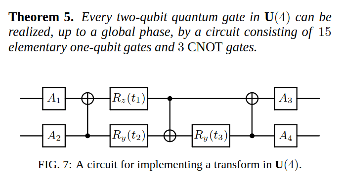
\text{CNOT} = |0\rangle\langle 0|\otimes \begin{pmatrix} 1 & 0\\ 0 &1\end{pmatrix} + |1\rangle\langle1 |\otimes \begin{pmatrix} 0 & 1\\ 1 &0\end{pmatrix}

https://arxiv.org/abs/quant-ph/0308006v3

=

2 qubit unitary

Canonical

KAK decomposition, Brockett's work etc

=

2 qubit unitaries modulo single qubit unitaries are a 3 dimensional torus

Quantum compiling

\(2\) qubits - \(4\times 4\) unitary matrix - use KAK decomposition + \(3\) CNOT formula

Quantum compiling

\(1\) qubit - \(2\times 2\) unitary matrix - use Euler angles

\(n\) qubits - \(2^n\) unitary matrix - use quantum Shannon decomposition + \(O(4^n)\) CNOT formula

Variational quantum eigensolver

https://arxiv.org/abs/quant-ph/0308006v3

0

+

This works but is inefficient

This is efficient but doesn't work

Open: fill this gap!

\hat W_k = [\hat D_{k-1},\hat H_{k-1}]

\hat H_k = e^{s_k \hat W_k} \hat H_{k-1} e^{-s_k \hat W_k}

Double-bracket iteration

s_k

Rotation durations:

Input:

\hat H_0

\hat D_k

Diagonal generators:

A new approach to diagonalization on a quantum computer

Great: we can diagonalize

How to quantum compile?

How to quantum?

Group commutator

\hat H \mapsto \hat \mathcal H_\ell = \hat \mathcal U_\ell^\dagger \hat H \hat\mathcal U_\ell

0

Want

\hat H_{k+1} = e^{s \hat W_k} \hat H_k e^{-s \hat W_k}

\hat W_k = [\hat D_k, \hat H_k]

e^{i\sqrt{s_k}\hat D_k}e^{i\sqrt{s_k}\hat H_k}e^{-i\sqrt{s_k}\hat D_k}e^{-i\sqrt{s_k}\hat H_k}= e^{-s[\hat D_k,\hat H_k]} +\hat E^\text{(GC)}

New bound

\|\hat E^\text{(GC)}\| \le 4\|\hat H_0\|\,\|[\hat D_k, \hat H_k]\| s^3

Group commutator during iteration

0

\hat H_{k} = \hat U_k^\dagger \hat H_0 \hat U_k

\hat V_0 = e^{i\sqrt{s_0}\hat D_0}e^{i\sqrt{s_0}\hat H_0}e^{-i\sqrt{s_0}\hat D_0}e^{-i\sqrt{s_0}\hat H_0}

e^{-it \hat H_{k} } = e^{-it \hat U_k^\dagger \hat H_0 \hat U_k}= \hat U_k^\dagger e^{-t \hat H_0} \hat U_k

\hat V_1 = e^{i\sqrt{s_1}\hat D_1}e^{i\sqrt{s_1}\hat H_{1}} e^{-i\sqrt{s_1}\hat D_1}e^{-i\sqrt{s_1}\hat H_{1}}

\hat U_k =\hat V_0 \hat V_1 \ldots \hat V_k

Group commutator during iteration

0

\hat H_{k} = \hat U_k^\dagger \hat H_0 \hat U_k

\hat V_0 = e^{i\sqrt{s_0}\hat D_0}e^{i\sqrt{s_0}\hat H_0}e^{-i\sqrt{s_0}\hat D_0}e^{-i\sqrt{s_0}\hat H_0}

e^{-it \hat H_{k} } = e^{-it \hat U_k^\dagger \hat H_0 \hat U_k}= \hat U_k^\dagger e^{-t \hat H_0} \hat U_k

\hat V_1 = e^{i\sqrt{s_1}\hat D_1}\hat V_{0}^\dagger e^{i\sqrt{s_1}\hat H_{0}}\hat V_0 e^{-i\sqrt{s_1}\hat D_1}\hat V_{0}^\dagger e^{-i\sqrt{s_1}\hat H_{0}}\hat V_0

\hat U_k =\hat V_0 \hat V_1 \ldots \hat V_k

\hat V_k = e^{i\sqrt{s_k}\hat D_k}\hat U_{k-1}^\dagger e^{i\sqrt{s_k}\hat H_{0}}\hat U_{k-1} e^{-i\sqrt{s_k}\hat D_k}\hat U_{k-1}^\dagger e^{-i\sqrt{s_k}\hat H_{0}}\hat U_{k-1}

\hat W_k = [\hat D_{k-1},\hat H_{k-1}]

\hat H_k = e^{s_k \hat W_k} \hat H_{k-1} e^{-s_k \hat W_k}

Double-bracket iteration

s_k

Rotation durations:

Input:

\hat H_0

\hat D_k

Diagonal generators:

A new approach to diagonalization on a quantum computer

Great: we can diagonalize

How to quantum compile?

Replace by the group commutator

e^{-s[\hat D_k,\hat H_k]}\approx e^{i\sqrt{s}\hat D_k}e^{i\sqrt{s}\hat H_k}e^{-i\sqrt{s}\hat D_k}e^{-i\sqrt{s}\hat H_k}

Group commutator iteration

\hat V_k = e^{i\sqrt{s_k}\hat D_k}e^{i\sqrt{s_k}\hat H_k}e^{-i\sqrt{s_k}\hat D_k}e^{-i\sqrt{s_k}\hat H_k}

\hat H_{k+1} = \hat V_{k}^\dagger\hat H_{k} \hat V_k

\hat V_{k} = e^{-s[\hat D_{k},\hat H_{k}]}

Double-bracket iteration

Transition from theory to QPUs

Follow

QIBO implementation

on Github

github.com/qiboteam/qibo/

How well does it work?

Variational flow example

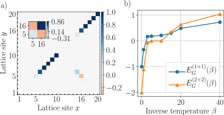
Notice the steady increase of diagonal dominance.

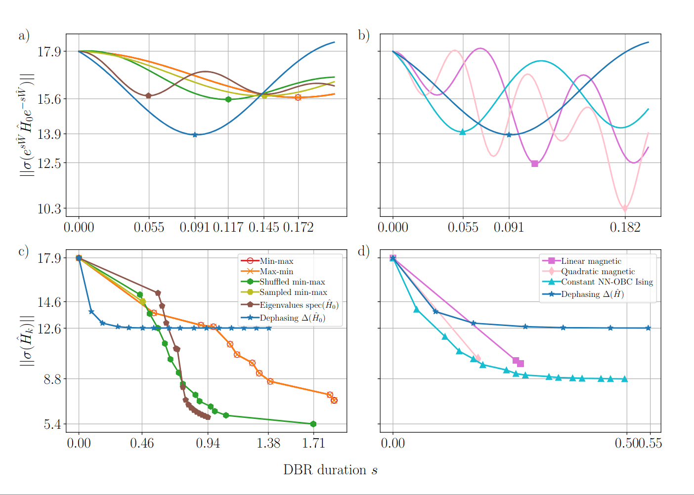
Variational vs. GWW flow

Notice that degeneracies limit GWW diagonalization but variational brackets can lift them.

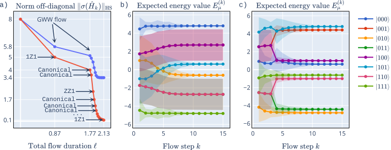
GWW for 9 qubits

Notice the spectrum is almost converged.

GWW for 9 qubits

Notice that some of them are essentially eigenstates!

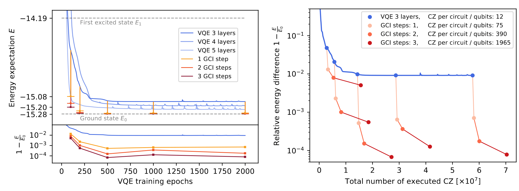
How does it work after warm-start?

10 qubit, 50 layers of CNOT - 99.5% ground state fidelity

\hat A_0 = \sum_{j=1}^L(X_j X_{j+1}+Y_j Y_{j+1}+ Z_j Z_{j+1})

https://arxiv.org/abs/2408.03987

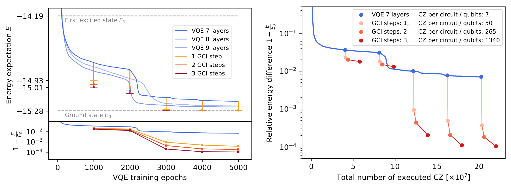
This both works and is efficient

How to interface VQE and DBQA?

Quantum Dynamic Programming

arxiv:2403.09187

with J. Son, R. Takagi and N. Ng

QDP code structure

Github PR #1302

Warm-start unitary from variational quantum eigensolver

0

+

=

= U_\theta

DBQA input with warmstart

\hat A_0 \rightarrow \hat H_0 = \hat U_\theta^\dagger \hat A_0 \hat U_\theta

V_0 = e^{i\sqrt{s_0}\hat D_0}e^{i\sqrt{s_0}\hat H_0}e^{-i\sqrt{s_0}\hat D_0}e^{-i\sqrt{s_0}\hat H_0}

V_0 = e^{i\sqrt{s_0}\hat D_0}\hat U_\theta^\dagger e^{i\sqrt{s_0}\hat A_0}\hat U_\theta e^{-i\sqrt{s_0}\hat D_0}\hat U_\theta^\dagger e^{-i\sqrt{s_0}\hat A_0}\hat U_\theta

Use unitarity and get circuit VQE insertions

10 qubit, 50 layers of CNOT - 99.5% ground state fidelity

\hat A_0 = \sum_{j=1}^L(X_j X_{j+1}+Y_j Y_{j+1}+ Z_j Z_{j+1}) \equiv \sum_{j=1}^L\hat A_0^{(j)}

e^{-it\hat A_0} \approx \left( \prod_{j=1}^L e^{-i t\hat A_0^{(j)}/M}\right)^M

e^{-i t\hat A_0^{(j)}/M}=

=

2 qubit unitary

Canonical

For quantum compiling we use:

higher-order group commutators
higher-order Trotter-Suzuki decomposition
3-CNOT formulas

New quantum algorithm for diagonalization

\hat H \mapsto \hat \mathcal H_\ell = \hat \mathcal U_\ell^\dagger \hat H \hat\mathcal U_\ell

\partial_\ell \hat \mathcal H_\ell = [[A(\hat \mathcal H_\ell),B(\hat \mathcal H_\ell)], \hat \mathcal H_\ell]

no qubit overheads

no controlled-unitaries

0

C

arXiv:2206.11772

0

Simple

=

Easy

Doesn't spark joy :(

Double-bracket quantum algorithm for diagonalization

\hat H \mapsto \hat H_\ell = \hat U_\ell^\dagger \hat H \hat U_\ell

\partial_\ell \hat H_\ell = [[A(\hat H_\ell),B(\hat H_\ell)], \hat H_\ell]

new approach to preparing useful states

0

arXiv:2206.11772

What else is there?

Linear programming

Matching optimization

Diagonalization

Sorting

QR decomposition

Toda flow

\partial_\ell \hat H_\ell = [[A(\hat H_\ell), B(\hat H_\ell)] , \hat H_\ell]

Double-bracket flow

Runtime-boosting heuristics

Analytical convergence analysis

Group commutator bound

Hasting's conjecture

Relation to other quantum algorithms

Code is available on Github

0

C

arXiv:2206.11772

Double-bracket quantum algorithms for diagonalization

arxiv:2403.09187

with J. Son, R. Takagi and N. Ng

\mathcal{E}^{(\mathcal{N},\rho,M)}_{QDP} \coloneqq (\mathcal{E}^{(\mathcal{N},\rho)}_{1/M})^M

Quantum dynamic programming

Material science?

0

C

arXiv:2206.11772

arxiv:1912.06076

arxiv:2005.09000

arxiv:1807.04567

How to dynamically quantum?

Group commutator

\hat H \mapsto \hat \mathcal H_\ell = \hat \mathcal U_\ell^\dagger \hat H \hat\mathcal U_\ell

\partial_\ell \hat \mathcal H_\ell = [[A(\hat \mathcal H_\ell),B(\hat \mathcal H_\ell)], \hat \mathcal H_\ell]

0

Want

\hat H_1 = e^{s \hat W_1} \hat H e^{-s \hat W_1}

\hat W_1 = [\Delta(\hat H),\sigma(\hat H)]

e^{is\Delta(\hat H)}e^{is\hat H}e^{-is\Delta(\hat H)}e^{-is\hat H}= e^{-s^2[\Delta(\hat H),\sigma(\hat H)]} +\hat E^\text{(GC)}

New bound

\|\hat E^\text{(GC)}\| \le 4\|\hat H\|\,\|[\Delta(\hat H),\sigma(\hat H)]\| s^3

Group commutator

\hat H \mapsto \hat \mathcal H_\ell = \hat \mathcal U_\ell^\dagger \hat H \hat\mathcal U_\ell

\partial_\ell \hat \mathcal H_\ell = [[A(\hat \mathcal H_\ell),B(\hat \mathcal H_\ell)], \hat \mathcal H_\ell]

0

Want

\hat H_1 = e^{s \hat W_1} \hat H e^{-s \hat W_1}

\hat W_1 = [\Delta(\hat H),\sigma(\hat H)]

e^{is\Delta(\hat H)}e^{is\hat H}e^{-is\Delta(\hat H)}e^{-is\hat H}= e^{- s^2[\Delta(\hat H),\sigma(\hat H)]} +\hat E^\text{(GC)}

How to get ?

\hat D_s(\hat H) \approx e^{is\Delta(\hat H)}

\hat C_s(\hat J) = \hat D_{\sqrt{s}}(\hat J)^\dagger \; e^{i\sqrt{s}\hat J}\; \hat D_{\sqrt{s}}(\hat J)\; e^{-i\sqrt{s}\hat J} \approx e^{-s \hat W(\hat J)}

1,

0,

0

Phase flip unitaries

\mu = (

)

N

S

N

S

N

S

N

S

\hat Z

\mathbb 1

\otimes

\hat Z

\mathbb 1

0,

1,

0,

1,

0,

1

\mu = (

)

1

\otimes

\mathbb 1

\otimes

\mathbb 1

\otimes

\hat Z

\otimes

1

\otimes

\mathbb 1

\otimes

\hat Z

\otimes

\hat Z

N

S

N

S

N

S

Phase flip unitaries

Evolution under dephased generators

\hat H \mapsto \hat H_\ell = \hat U_\ell^\dagger \hat H \hat U_\ell

\partial_\ell \hat H_\ell = [[A(\hat H_\ell),B(\hat H_\ell)], \hat H_\ell]

0

\hat Z_\mu e^{-i s \hat J} \hat Z_\mu = e^{-is \hat Z_\mu \hat J\hat Z_\mu}

\hat D_s(\hat J) \approx \prod_{\mu\in R} \hat Z_\mu e^{-i s \hat J/D} \hat Z_\mu

We can make it efficient:

\Delta(\hat J)= \frac 1 {\dim (\hat J)} \sum_{\mu\in\{0,1\}^{\times L}} \hat Z_\mu \hat J \hat Z_\mu

R \subseteq \{0,1\}^{\times L}

Use unitarity

and repeat many times

New quantum algorithm for diagonalization

\hat H \mapsto \hat \mathcal H_\ell = \hat \mathcal U_\ell^\dagger \hat H \hat\mathcal U_\ell

\partial_\ell \hat \mathcal H_\ell = [[A(\hat \mathcal H_\ell),B(\hat \mathcal H_\ell)], \hat \mathcal H_\ell]

0

arXiv:2206.11772

\hat D_s(\hat J) = \prod_{\mu\in\{0,1\}^{\times L}} \hat Z_\mu e^{-i s \hat J/D} \hat Z_\mu

\hat C_s(\hat J) = \left( \hat D_{\sqrt{2s/K}}(\hat J)^\dagger \;e^{i\sqrt{2s/K}\hat J}\;\hat D_{\sqrt{2s/K}}(\hat J)\;e^{-i\sqrt{2s/K}\hat J}\right)^K

\hat V_k = \hat V_{k-1}\hat C_s(\hat J_{k-1})

\hat J_{k-1} = \hat V_{k-1}^\dagger \hat H \hat V_{k-1}

1) Dephasing

2) Group commutator

3) Frame shifting

\partial_\ell \hat \mathcal H_\ell = [[A(\hat \mathcal H_\ell),B(\hat \mathcal H_\ell)], \hat \mathcal H_\ell]

\hat V_k = \hat C_s(\hat J_{1})\; \hat C_s(\hat J_{2})\ldots \hat C_s(\hat J_{k-1}) \approx e^{-s \hat W_1}\;e^{-s \hat W_2}\ldots e^{-s \hat W_{k-1}}

Euler's fundamental discoveries about the exponential function: Their role in quantum computing

Click links at slides.com/marekgluza

Sums and infinite sums

Sums and infinite sums

Sums and infinite sums

The exponential function

Quantum mechanics

Quantum mechanics

Braket notation

Using Euler's formula to 'program a qubit

Infinite products

Double-bracket quantum algorithms for diagonalization

slides.com/marekgluza

Experimental Observation of Curved Light-Cones in a Quantum Field Simulator

Breaking of Huygens-Fresnel principle in inhomogeneous Tomonaga-Luttinger liquids

Tomography for phonons

Quantum mechanics

Examples of infinite sums

Quantum mechanics

Quantum mechanics

Why double a bracket?

Why double a bracket?

Inspired by double-bracket flows we compiled quantum circuits which yield quantum states relevant for material science

Double-bracket rotation ansatz

Double-bracket rotation ansatz

Double-bracket rotation ansatz

Double-bracket rotation ansatz

Double-bracket iteration

Głazek-Wilson-Wegner flow

as a quantum algorithm

Głazek-Wilson-Wegner flow

as a quantum algorithm

New quantum algorithm for diagonalization

What about other methods?

Double-bracket iteration

How to quantum?

Group commutator

Want

New bound

Group commutator during iteration

Group commutator during iteration

Double-bracket iteration

Group commutator iteration

Double-bracket iteration

Double-bracket iteration

Transition from theory to QPUs

Follow

QIBO implementation

on Github

How well does it work?

Variational flow example

Variational vs. GWW flow

GWW for 9 qubits

GWW for 9 qubits

How does it work after warm-start?

How to interface VQE and DBQA?

Quantum Dynamic Programming

QDP code structure

New quantum algorithm for diagonalization

Double-bracket quantum algorithm for diagonalization

What else is there?

Linear programming

Matching optimization

Diagonalization

Sorting

QR decomposition

Toda flow

Double-bracket flow

Runtime-boosting heuristics

Analytical convergence analysis

Group commutator bound

Hasting's conjecture

Relation to other quantum algorithms

Code is available on Github

Double-bracket quantum algorithms for diagonalization

Material science?

How to dynamically quantum?

Group commutator

Want

New bound