

Data Science
Data Science
-
Introduction to Pandas -
Plotting Data -
Getting Data
Intoduction to Pandas
- Python Library
- Used for Analysing data

Chapter 1 | Intro to Pandas
import pandas as pd # importing the module

df = pd.DataFrame( # hard-coding a data-frame
    [['Jan', -18, 2],
    ['Jul', 32, 18],
    ['Dec',-12, 7]],
    index = [0,1,2], # index values
    columns = ['month', 'lowest_temp', 'highest_temp']) # column names

print df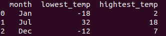
Code example for returning a Data frame
Indentation
- Python Indentations (Exc 2)
Where in other programming languages the indentation in code is for readability only, in Python the indentation is very important.
Python uses indentation to indicate a block of code.
Chapter 1 | Python, class intro
Indentation
- Python Indentations (Exc 2)
Where in other programming languages the indentation in code is for readability only, in Python the indentation is very important.
Python uses indentation to indicate a block of code.
Chapter 1 | Python, class intro
Data Science
Chapter 1 | Intro to Pandas

Data Science
Chapter 1 | Intro to Pandas
Data Science
Chapter 1 | Intro to Pandas
-
Can include many layers of data
-
Often, you will only work with a few layers at one time
- You can exclude your code from returning all the layers
print df['highest_temp']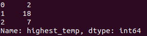
Plotting Data
Chapter 2 | Plotting Data
Scatter plot
Chapter 2 | Plotting Data
import numpy as np
import matplotlib.pyplot as plt

x = np.array([0, -3, 6, 4])
y = np.array([2, 4, 3, 1])

plt.scatter(x,y)
plt.savefig('/usercode/myfig')
plt.show()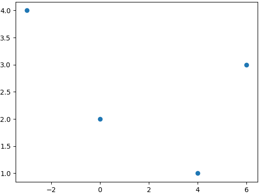
Graph plot
Chapter 2 | Plotting Data
import matplotlib.pyplot as plt
import numpy as np

x = np.linspace(-5,5,50)

def y():
    return x**2

plt.plot(x,y(x))
plt.savefig('/usercode/myfig')
plt.show()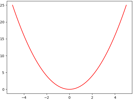
- np.linspace(-5, 5, 50) will make an array with 50 elements between -5 and 5
Plotting data
Chapter 2 | Plotting Data
- One more example with plotting, but this time with Pandas
import pandas as pd
import matplotlib.pyplot as plt

# Tracking height [m] of a young person

df = pd.DataFrame(
    [[2018,160],
    [2019,164],
    [2020,168],
    [2021,171],
    [2022,173],
    [2023,176],
    [2024,178],
    [2025,179],
    [2026,180],
    [2027,180]],
    index = [0,1,2,3,4,5,6,7,8,9],
    columns = ['year', 'height'])

plt.plot(df.year, df.height)
plt.savefig('/usercode/myfig')
plt.show()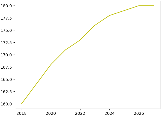
Getting Data
Chapter 3 | Getting Data
Getting Data
Chapter 3 | Getting Data
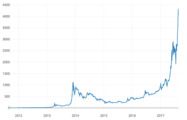
- Use what we have learn in a real world application.
- Extracting data from the web
- Plotting and analysing the Bitcoin Price Index
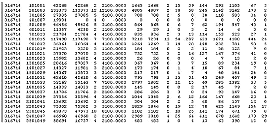
Reading datafiles
Chapter 3 | Getting Data
- You can also extract data from datafiles making the process faster
import pandas as pd

prices = pd.read_csv('bitCoinPrices2010To2018.csv')
df = DataFrame(prices)
Reading datafiles
Chapter 3 | Getting Data
- You could also read data directly form the web.
import pandas as pd
import requests
r = requests.get('https://api.coindesk.com/v1/bpi/historical/close.json?start=2013-01-01&end=2014-01-01')

df = pd.DataFrame(r.json())- Soon, you are going to use this script to plot the change in Bitcoin price over time
Processing and Graphing Data
Chapter 4 | Processing and Graphing Data
- More matplotlib to add information
- Use that information to generate more readable graphs
Processing and Graphing Data
Chapter 4 | Processing and Graphing Data
# Variation in velocity for a car on a given highway
plt.plot(df1.vel, df1.time, '-r') # Red plot

# Variation in velocity for a truck on a given highway
plt.plot(df2.vel, df2.time, '-b') # Blue plot

plt.xlabel('time (s)') # x-axis indicates time in seconds
plt.ylabel('velocity (m/s)') # y-axis indicates velocity in m/s
plt.title('Tracking velocity for a car and a truck on a highway')
plt.legend(['Car', 'Truck'])
plt.show()
Example of more implementation with matplotlib
Methods for getting the speed at any given time
# printing the speed
# after 5 seconds
print pf1.vel[4]

# Printing highest
# speed reached
print pf1.max()
BitCoin price prediction
Chapter 5 |BitCoin price prediction
BitCoin price prediction
Chapter 5 |BitCoin price prediction
-
This and next chapter: More familiar with what you can do with bitcoin data
-
Learning about normalization
- Using a prebuilt script to predict BPI
BitCoin price prediction
Chapter 5 |BitCoin price prediction
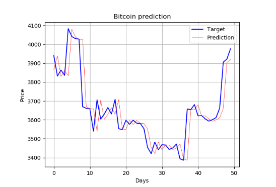
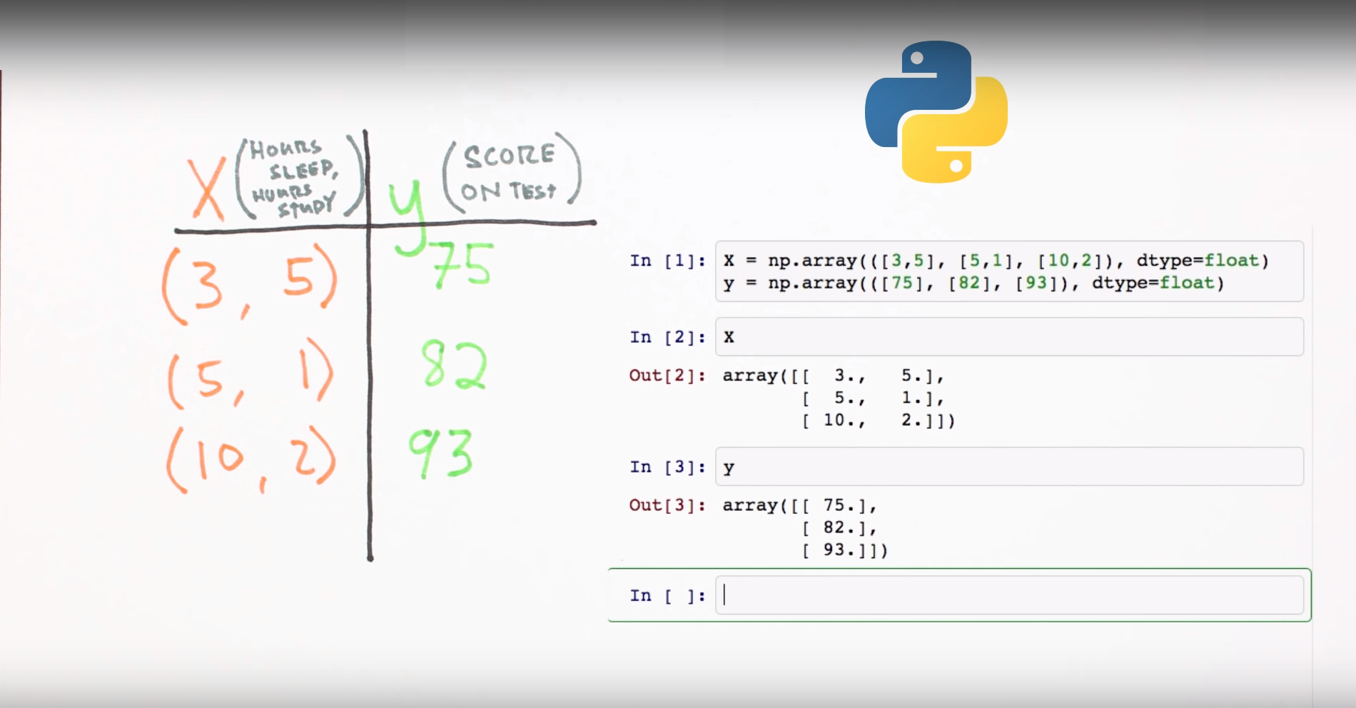
- A prebuilt Neural Network in Exercise 1 that predicts the BPI
- Target value = The real Bitcoin price
- Predicted value = The price predicted by our Neural Network
BitCoin price prediction
Chapter 5 |BitCoin price prediction
Convert a list to a Numpy array
import numpy as np

NewArray = np.asarray(list)
BitCoin price prediction
Chapter 5 |BitCoin price prediction
When should you buy or sell?
Chapter 6 |Investment

When should you buy or sell?
Chapter 6 |Investment
-
When should you buy or sell BitCoins?
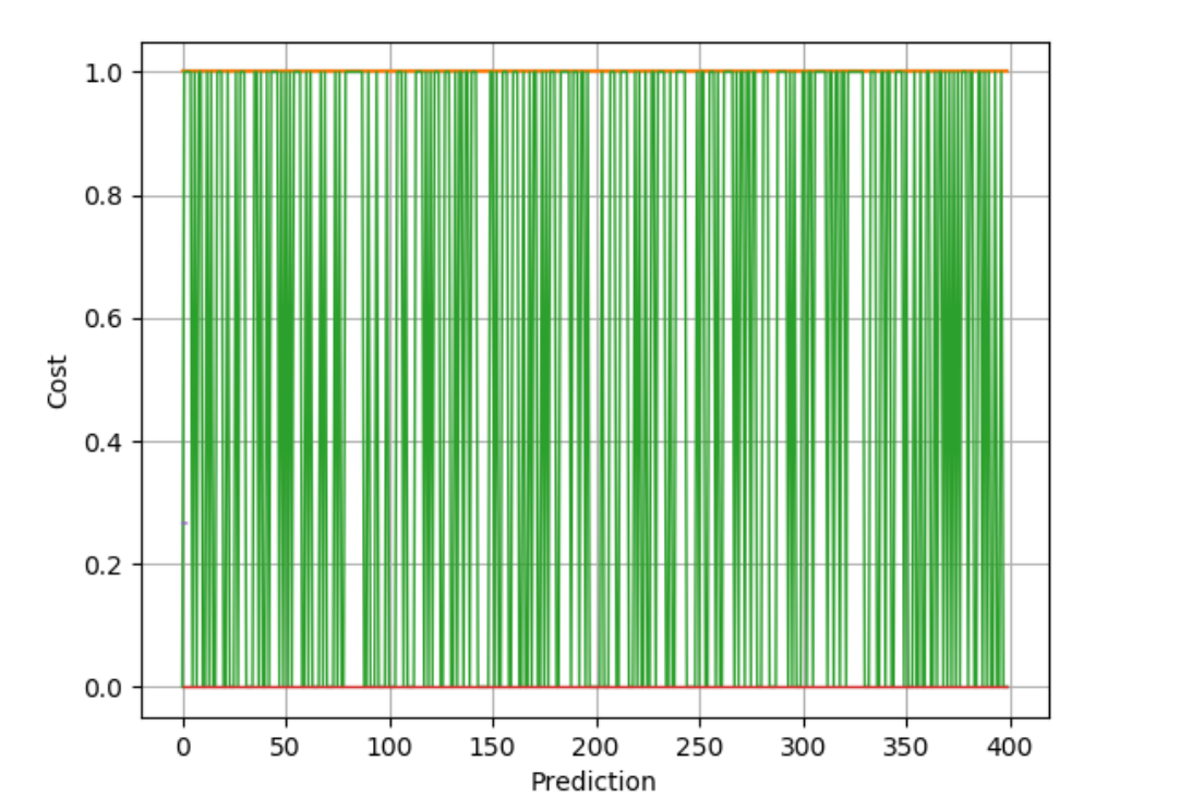
- Normalization helps for predicting when you should invest!
- Gives the output a value
between 0 and 1
def prepareDF(data):
    x_normed = data/ data.max(axis=0)
    return x_normed
1 = Sell Bitcoins
0 = buy BitCoins
When should you buy or sell?
Chapter 6 |Investment
Training our Neural Network
def createTrain(dataset, array):
    for i in range(len(dataset)-(len(dataset)//5)):
        currentdata = dataset[i]['close']
        previousdata= dataset[i-1]['close']
        array.append([dataset[i]['close'], dataset[i]['volumeto'],
        dataset[i]['volumefrom'],currentdata-previousdata])
    NewArray = np.asarray(array)
return prepareDF(NewArray)- We create a function
that uses 20% of the
values in the
dataframe
- TrainOutput func
that gives us a
value between
0 and 1
When should you buy or sell?
Chapter 6 |Investment
Test input
def createTestInput(dataset, array):
    length = 4*(len(dataset))//5
    for i in range(len(dataset)-length):
        currentdata = dataset[length+i]['close']
        previousdata= dataset[length+i-1]['close']
        array.append([dataset[i]['close'], dataset[i]['volumeto'],
        dataset[i]['volumefrom'],currentdata-previousdata])
    NewArray = np.asarray(array)
return prepareDF(NewArray)- Uses 80% of the values
in the df
- Has also testOutput
that returns a value
between 0 and 1
When should you buy or sell?
Chapter 6 |Investment
Linear Algebra for Data Science
Chapter 1 | Basic Vector operations Data

Linear Algebra for Data Science
Chapter 1 | Basic Vector operations Data
- A vector is list of elements with the elements listed either vertically or horizontally
- A vector with vertical elements is called a column vector, while one with horizontal elements is called a row vector
import numpy as np

# Making a vector
v = np.array([2,-3,1,0])
Transpose of a vector
Chapter 1 | Basic Vector operations Data
- A row vector transposed is the same vector turned 90 degrees.
- A column vector transposed will become a row vector and vice versa!
vT = np.transpose(v)Linear Algebra for Data Science
Chapter 1 | Basic Matrix operations Data
| height | weight | vertical | sprint | |
|---|---|---|---|---|
| 1 | 196 | 98 | 40 | 6.4 |
| 2 | 205 | 124 | 34 | 6.7 |
| 3 | 198 | 115 | 36 | 6.6 |
| 4 | 192 | 107 | 38 | 6.3 |
| 6 | 208 | 127 | 35 | 6.7 |
List of data, i.e stats for a group of Basketball players
Can be represented as a matrix
Linear Algebra for Data Science
Chapter 1 | Basic Matrix operations Data
- The transpose is found the same way in a matrix
- Coding a matrix is just as easy as coding a vector
import numpy as np

M = np.array([[1, 3, -2], [0, -2, 5], [3, 0, -1]])
MT = np.transpose(M)Matrix-Vector operations
Chapter 3 | Matrix-Vector operations
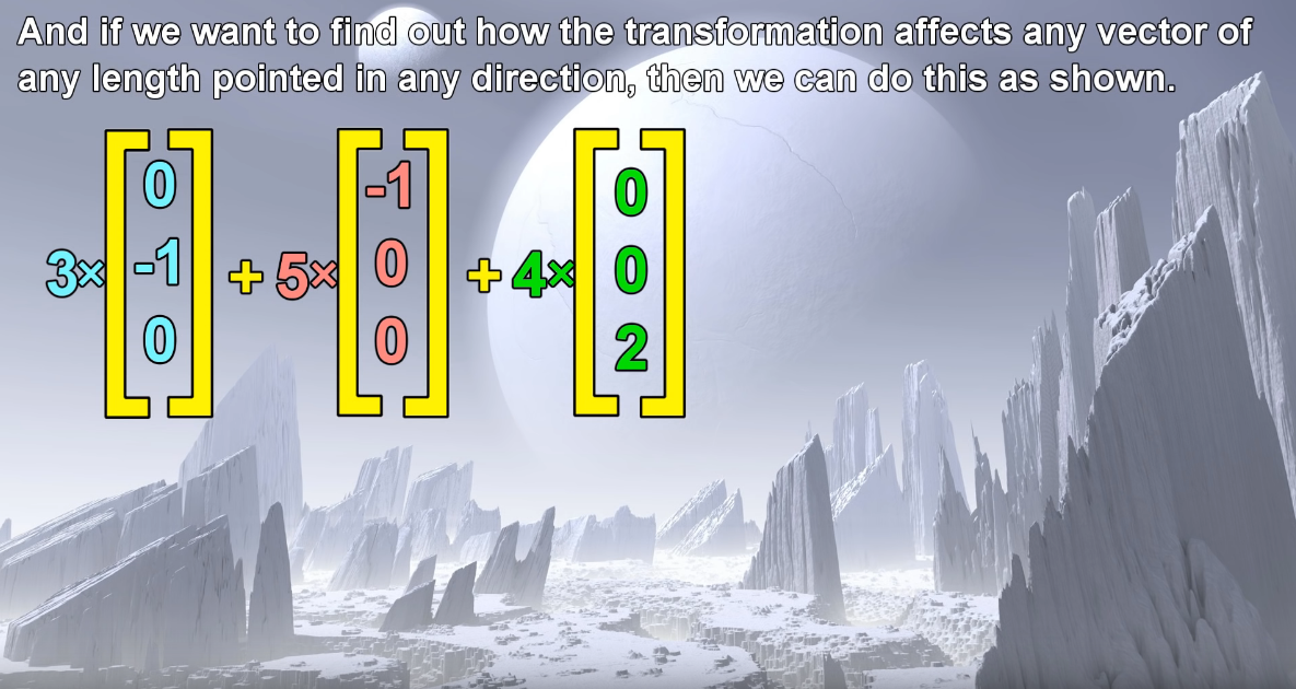
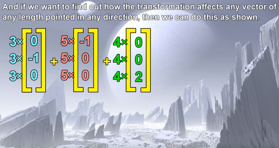
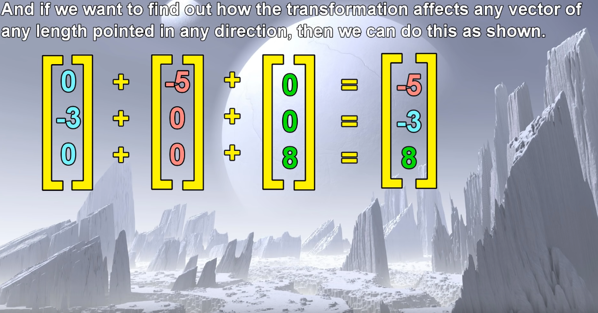
- How to multiply Matrices with Vectors
- Which matrices and vectors can be multiplied with each other?
Matrix-Vector operations
Chapter 3 | Matrix-Vector operations
2x2 Matrix
2x1 Vector
Output 2x1 vector
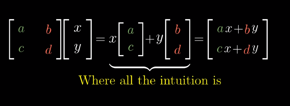
Multiplying a matrix with a vector
Chapter 3 | Matrix-Vector operations
Multiplying a matrix with a vector
Chapter 3 | Matrix-Vector operations
Matrix-Matrix Multiplication
Chapter 4 | Matrix-Matrix multiplication
- Matrix-Matrix multiplication
- Which matrices can be multiplied together?
- The Identity matrix
Matrix-Matrix Multiplication
Chapter 4 | Matrix-Matrix multiplication
The number of columns in matrix A
needs to be the same as the rows in matrix B
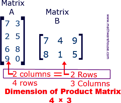
The output matrix will have rows same as matrix A and columns same as matrix B
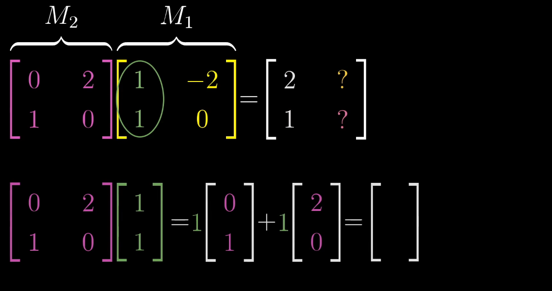
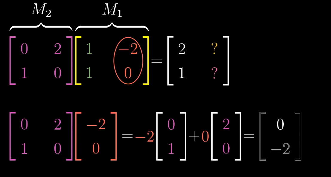
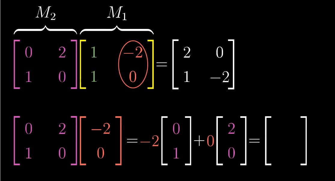
Matrix-Matrix Multiplication
Chapter 4 | Matrix-Matrix multiplication
As you can see. Multiplying matrices manually can be a long, tedious process
Luckly, This process can be done with just one line in Python!
np.dot(A, B)Matrix-Matrix Multiplication
Chapter 4 | Matrix-Matrix multiplication
Matrix-Matrix Multiplication
Chapter 4 | Matrix-Matrix multiplication
Matrix-Matrix Multiplication
Chapter 4 | Matrix-Matrix multiplication
Matrix-Matrix Multiplication
Chapter 4 | Matrix-Matrix multiplication
- It is important to notice that when doing Matrix-Matrix multiplication. A * B is not same as B * A
- Why do you think it is that way?
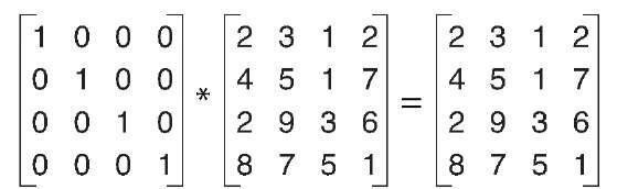
The Identity Matrix
Chapter 4 | Matrix-Matrix multiplication
- The only matrix that has the property that a matrix multiplied with it, returns the original matrix
- The Identity matrix, I, is square, meaning it always has the same number of rows and columns
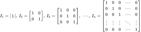
The Identity Matrix
Chapter 4 | Matrix-Matrix multiplication
Can be coded like this:
import numpy as np

# Making the 3x3 Identity matrix in two ways

# First way
I = np.array([[ 1.,  0.,  0.], [ 0.,  1.,  0.], [ 0.,  0.,  1.]])

# Second Way
I = np.identity(3)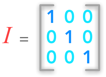
Which matrixes can be multiplied
Chapter 4 | Matrix-Matrix multiplication
Size of new matrix after multiplication
Chapter 4 | Matrix-Matrix multiplication
Matrix multiplication
Chapter 4 | Numpy
Matrix multiplication
Chapter 4 | Numpy
Matrix multiplication
Chapter 4 | Numpy
Matrix multiplication
Chapter 4 | Numpy
Matrix multiplication
Chapter 4 | Numpy
Matrix multiplication
Chapter 4 | Numpy
Matrix multiplication
Chapter 4 | Numpy
Matrix multiplication
Chapter 4 | Nempy
Matrix multiplication
Chapter 4 | Numpy
Matrix multiplication
Chapter 4 | Numpy
Matrix multiplication
Chapter 4 | Numpy
Matrix multiplication
Chapter 4 | Numpy
Matrix multiplication
Chapter 4 | Numpy
Create a Class
To create a class, use the keyword class:
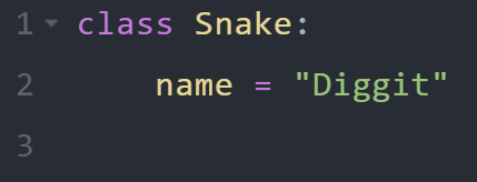
Example
Create a class named Snake, with a property named name
Chapter 1 | Python, class intro
The __init__() Function
Use the __init__() function to assign values to object properties, or other operations that are necessary to do when the object is being created.
Chapter 2 | More on classes
The __init__() Function
In the class named Snake, use the __init__() function to assign values for new_color
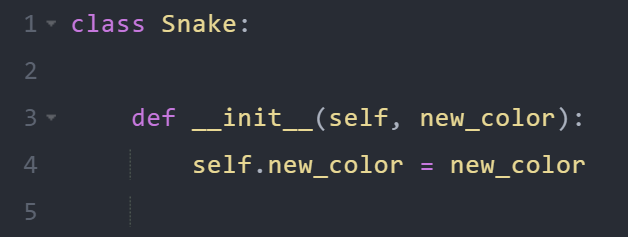
Example
Chapter 2 | More on classes

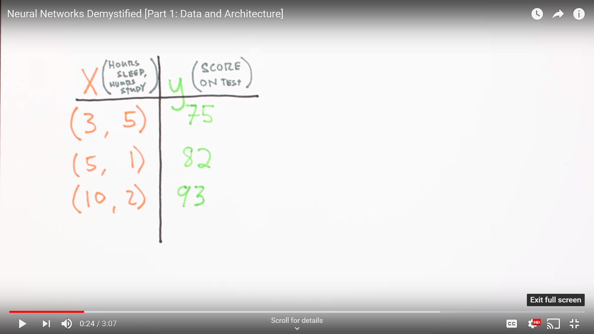
Data architecture
Chapter 3 | What’s a Neural Network?
Chapter 3 | What’s a Neural Network?
Chapter 3 | What’s a Neural Network?
What does this look like in code format using Numpy?
Chapter 3 | What’s a Neural Network?
Chapter 3 | What’s a Neural Network?
Chapter 3 | What’s a Neural Network?
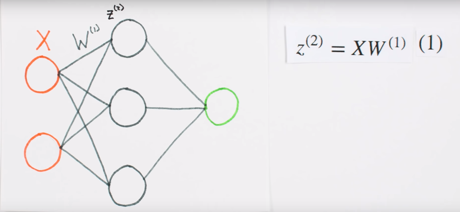
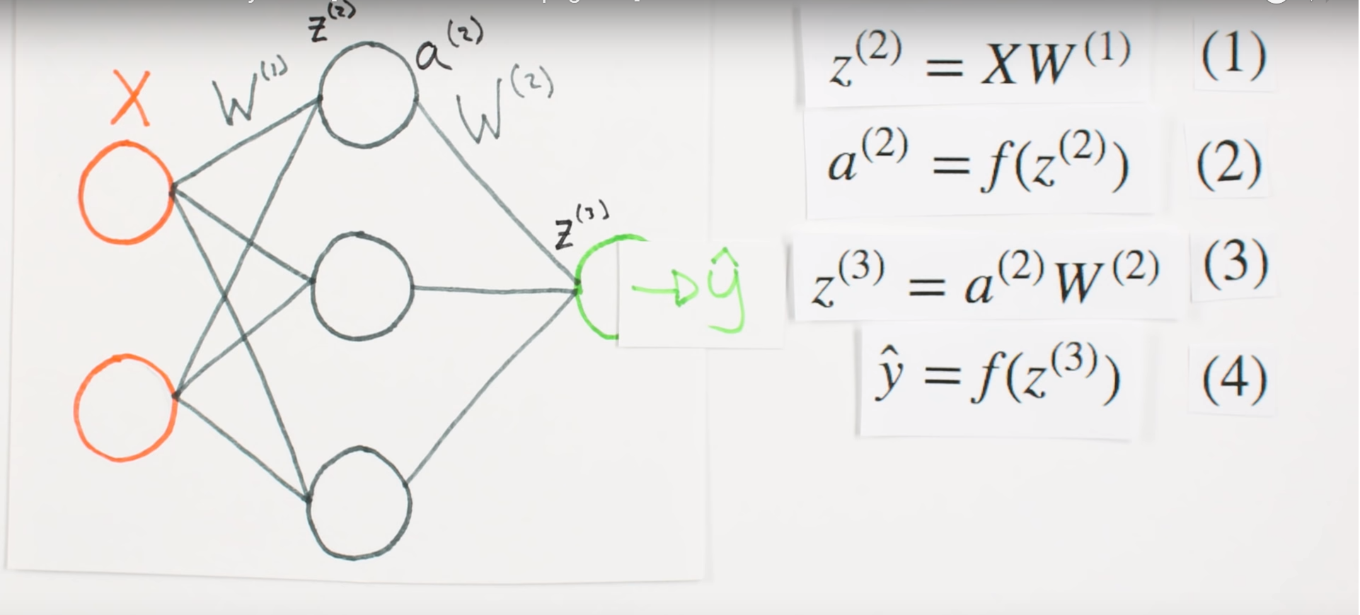
Forward propagation Intro
Chapter 5 | Forward propagation Intro
Chapter | Forward propagation Intro
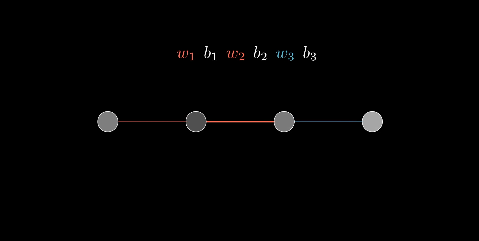
Multiplication
of layers and weight matrices
Chapter | Forward propagation Intro
Multiplication
of layers and weight matrices
Chapter | Forward propagation Intro
Chapter | Forward propagation Intro
Chapter | Forward propagation Intro
Chapter | Forward propagation Intro
Multiplication
of layers and weight matrices
Chapter | Forward propagation Intro
Multiplication of layers and weight matrices
Chapter | Forward propagation Intro
Multiplication of layers and weight matrices
Chapter | Forward propagation Intro
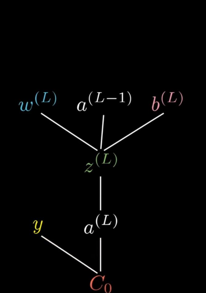
What they represent mathematically
Chapter | Forward propagation Intro
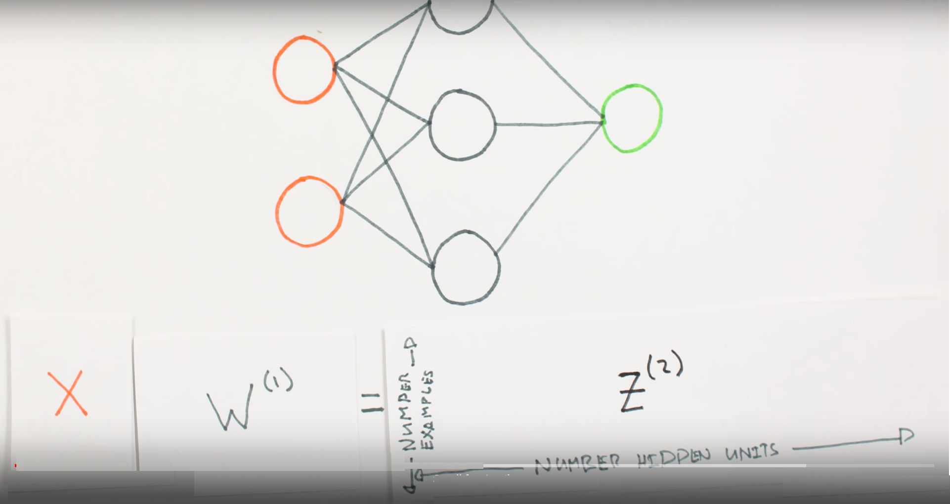
What is Z representing
Chapter | Forward propagation Intro

What we learned
Chapter | Sigmoid Function
Sigmoid Function
Chapter | Sigmoid Function
We need to convert our values into a probable value
Chapter | Sigmoid Function
Chapter | Forward Propagation Continued
Chapter | Forward Propagation Continued
Bootcamp- Concepts
www.diggitacademy.co.uk
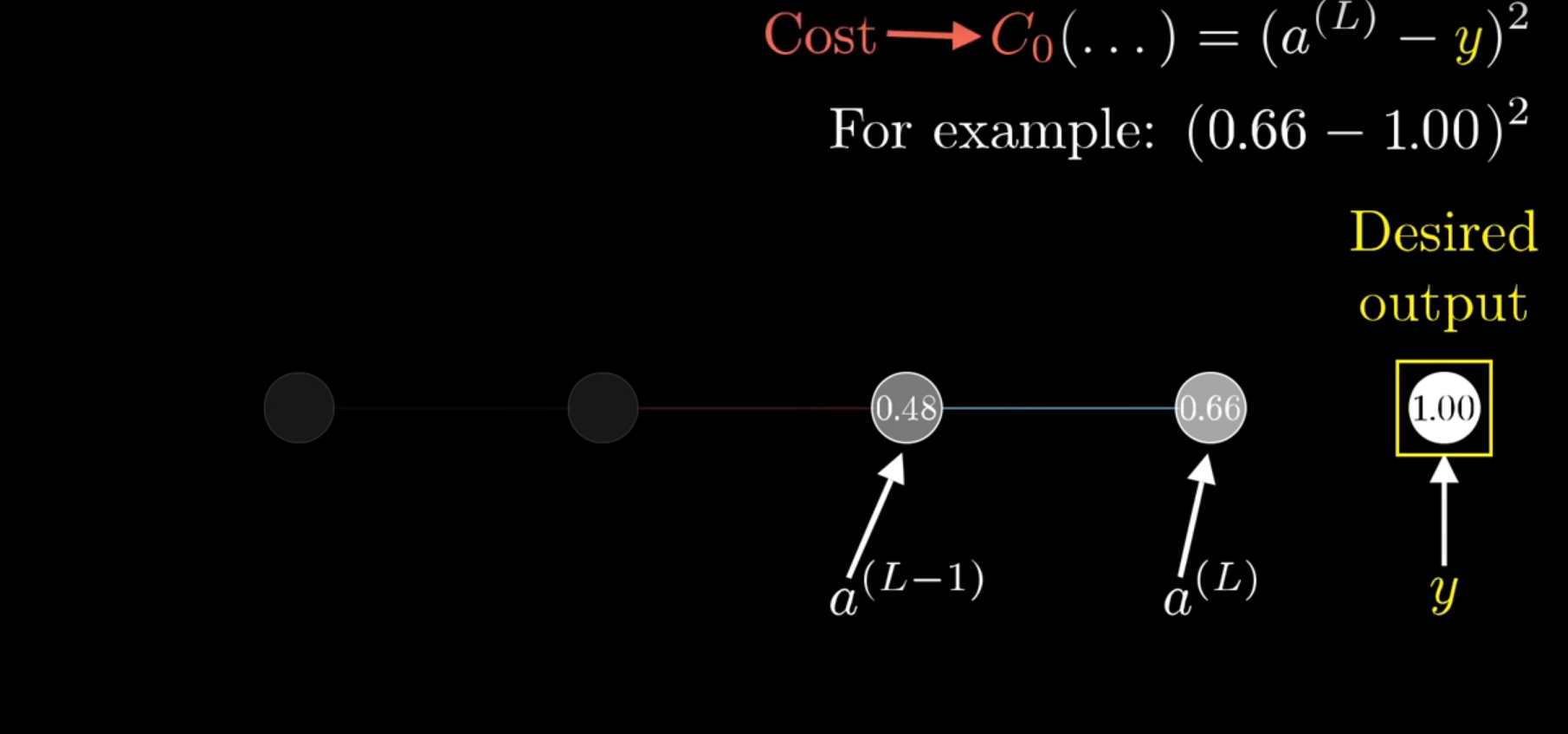
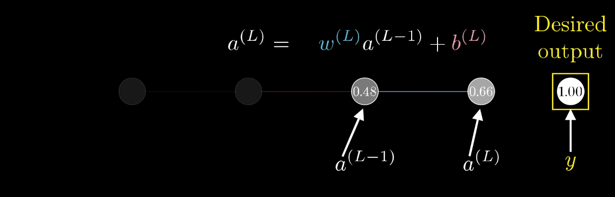
Chapter | Error Calcuation
Chapter | Error Calcuation
Chapter | Error Calcuation

Chapter | Error Calcuation

Chapter | Error Calcuation
Chapter | Error Calcuation

https://www.surveymonkey.com/r/QY2W2C9
Please give us feedback :)
There are only 5 questions in the Survey
Linear Regression