Monitoring
Data analyzis - noise, incertainity, optimization
INSEP | 03.04.2019
UE7 - Accompagnement scientifique à la Performance
Mathieu Lacome | @mathlacome
"One key area of evolution may be the use of data that is available from applied Soccer science support programmes. These developments likely occur through the more eFFective use of existing data steams in addition to the analysis and interpretation of new inputs."
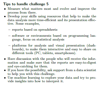
CHALLENGE 5
HANDLING THE DATA TSUNAMI
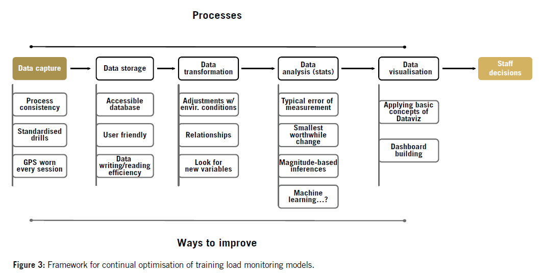
DATA STORAGE
How to store data in excel spreedsheets?
DATA TRANSFORMATION
How learning to code could save your life?
DATA ANALYSIS
Finding the signal within all this noise
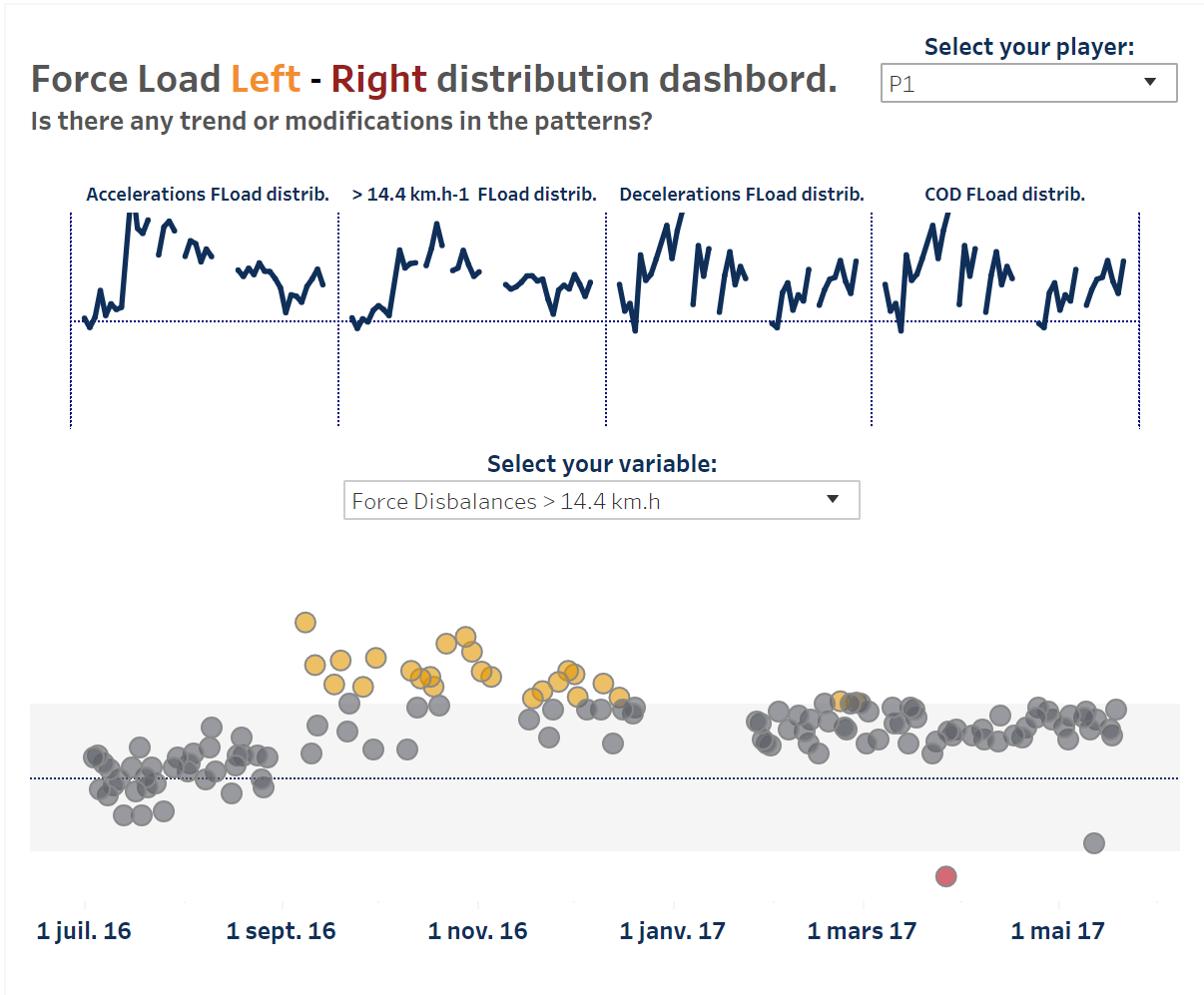
DATA VISUALISATION
Lets make it sexy
DATA STORAGE

highly recommended reading!
1. BE CONSISTENT
"Whatever you do, do it consistently."
2. USE GOOD NAMES FOR THINGS
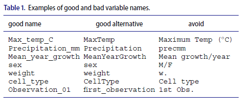
"AS A GENERAL RULE, DO NOT USE SPACES, EITHER IN VARIABLE NAMES OR FILE NAMES."
3. WRITE dates as yyyy-mm-dd
Excel worksheet that are going to contain dates, so that it does not do anything to them. To do this:
-
Select the column
-
In the menu bar, select Format→ Cells
-
Choose “Text” on the left
"WHEN ENTERING DATES, USE “ISO 8601” STANDARD, YYYY-MM-DD, SUCH AS 2013-02-27."
4. Put just one thing in a cell
"The cells in your spreadsheet should each contain one piece of data. Do not put more than one thing in a cell."
| name_id | height | size |
|---|---|---|
| 1 | 180 | M |
| 2 | 170 | L |
5. Make it a rectangle
"The best layout for your data within a spreadsheet is as a single big rectangle with rows corresponding to subjects and columns corresponding to variables. The first rowshould contain variable names, and please do not use more than one row for the variable names."
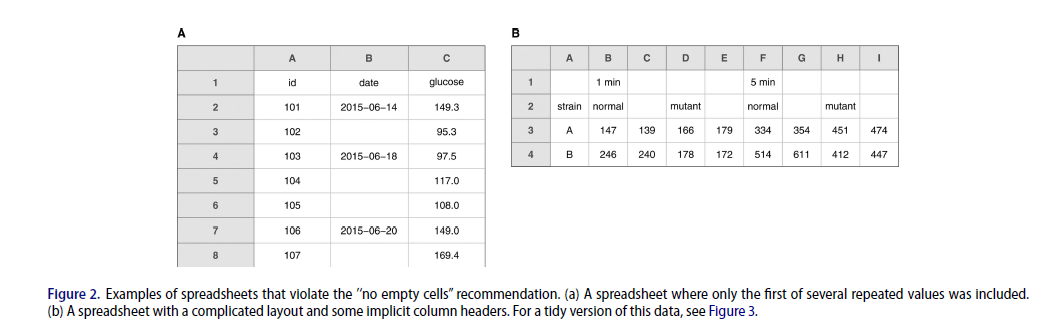
5. Make it a rectangle
6. create a data dictionary
-
The exact variable name as in the data file
-
A version of the variable name that might be used in data
visualizations
-
A longer explanation of what the variable means
-
The measurement units
-
Expected minimum and maximum values
7. Data & nothing else
-
no calculations
-
NO COLORS
-
nothing else than data
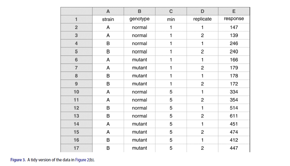
Quick exemple
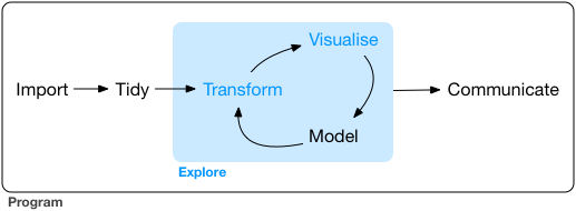
data transformation
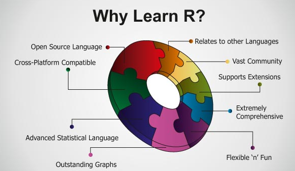
HOW R SAVE MY LIFE!
How R can save some time to:
library(readr)
library(tidyr)
library(lubridate)
library(purrr)
library(dplyr)
library(ggplot2)

setwd("C:/Users/mlacome/Documents/PeakIntensity")


### ICI ON PRESET LES VALEURS QUE L'ON SOUHAITE 'CUTTER' ###

TD_cut = 150
V2_cut = 20
MW_cut = 2
#########################
start_time <- Sys.time()

### Importer les fichiers présents dans ce dossier ###
temp <- list.files(path = "Data", pattern="*.csv", full.names = TRUE)
my_file <- map_dfr(temp, read_csv, col_types = cols(`cL/min` = col_double(),
                                                `vL/min` = col_double(),
                                                `fL/min` = col_double(),
                                                maxA = col_double(),
                                                maxD = col_double(),
                                                maxV = col_double(),
                                                `HR1%` = col_double(),
                                                `HR2%` = col_double(),
                                                maxV = col_double(),
                                                `VC Impulse Total/min` = col_double()),
               .id = "FileName") %>%
  dplyr::mutate(Key = paste(Date, Surname, Code, sep = "-")) %>%
  unique()
Importing multiple csv. into 1 database
How R can save some time to:
library(tidyverse)
library(readxl)

Master_FION <- read_excel("C:/Users/mlacome/Dropbox/1_Dropbox PSG/gps/Master/Master GPS ww new (040716).xlsm", sheet="Data")

Master_Meunier <- Master_FION %>%
  filter(Surname == "Meunier") %>%
  filter(Mode == "G") %>%
  filter(`Drill Category` == "1stHalf" | `Drill Category` == "Game") %>%
  filter(Club == "PSG") %>%
  select(Surname, `Drill Category`, Club, `Friendly date`, Dur, Vol, V1, V2, Spr, `Acc#Total`, `Acc(m)Total`, `Dec#Total`, `Acc(m)Total`, maxV, maxA, maxD) %>%
  mutate(Inf_V1 = Vol - V1,
         V2_V1 = V1 - V2,
         Spr_V2 = V2 - Spr)

write.xlsx2(Master_Meunier, file = "Master_Meunier.xlsx")
HANDLING multiple transformation
How R can save some time to:
R Markdown - the lab notebook 2.0
How R can save some time to:
R Markdown - the lab notebook 2.0
---
title: "Peak_Intensity_INSEP"
author: "Lacome M."
date: "2 avril 2019"
output: html_document
---

One of the challenges to assess match demands is that the intensity and density of actions is likely time-independent, i.e., the longer the period, the lower the average intensity. [Delaney et al.](https://www.researchgate.net/publication/315750153_Modelling_the_decrement_in_running_intensity_within_professional_soccer_players) proposed to model match-related locomotor intensity vs. time relationship during matches using a power relationship. We used this method in a [recent paper](http://mathlacome.rbind.io/publication/2017-ssg-football/) to examine at which extent different SSG formats could be used to either under- or overload the running- and/or mechanical- demands of competitive matches. In this post, we will see how to perform these analyses in R.

```{r message=FALSE, warning=FALSE}
library("tidyverse")
library("readxl")
library(RcppRoll)
```

First, I need to import csv files to create my database. To work around these models, we usually use multiple csv. An easy and efficient way to import a batch of files is to *map* the *read_csv* function over the differents files.

For this, the first step is to list all the files into our directory and then path the list of files as an argument to the function read_csv with the map function from the purrr package.

```{r warning=FALSE}


my_files <- list.files(path = "C:/Users/mlacome/Documents/MathLacome-2018-blog/1_DataSets/0_GameData", pattern="*.csv", full.names = TRUE)
my_file <- map_dfr(my_files, read_csv, skip = 2, .id = "FileName")
head(my_file)

```

We imported tracking data with only Players x & y positions. Using mutate, we can calculate distances, speeds & thus, distances covered in different speed zones.
data analysis
FINDING THE SIGNAL WITHIN ALL THIS NOISE
DATA VISUALISATION