Numerical modeling of stochastic Lie transport in fluid dynamis
based on the paper of prof. Dan Crisan et al., 2018,
Imperial College, London
Introduction
Challenges in weather forcasting and climate change predictions
- measurement errors
- measurement uncertainty
Modeling:
due to:
- incomplete data
- incomplete theoretical knowledge
Data driven models
- values and uncertainty of future measures
Predict:
based on:
- input of measures and statistical anaysis of the initial data
Data assimilation: "in flight corrections" allows Numerical weather predictions
A stochastic framework for a data-driven model
- introduction of noise should preserve the fundalmental mathematical structure of the deterministic model
- Why consider the SALT equations:
- not aiming to resolve the unresolved scales to predict their effects increasing the resolution
- whereas, using the spatial correlation of the datas to model the effect of the uncertainty as spatially correlated stochastic transport
- not aiming to resolve the unresolved scales to predict their effects increasing the resolution
3D Euler SALT equations


divergence free vector fields to be determined from the data
is the vorticity field
Emprical Orthogonal Functions (EOF)
Numerically (fine-coarse grid)
Uncertainty quantification (UQ) using SALT
- Fine grid Lagrangian trajectories (deterministic PDE)
- Coarse grid Lagrangian trajectories (deterministic PDE -spatially filter velocity)
- Difference between fine-coarse grid trajectory on non-overlappling time intervals (velocity-velocity correlation tensors)
- Velocity-velocity correlation tensors substitute in SALT to perform UQ
2D Euler SALT equations on a square
2D Euler equations: deterministic
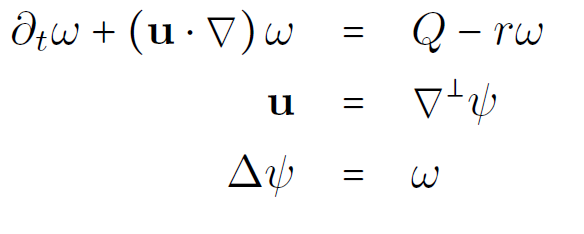

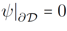
forcing
boundary condition

damping rate
Numerical scheme
-
SPACE: Galerkin finite elements
-
TIME: 3rd order Runge-Kutta
Bernsen et al. [2006]; Gottlieb [2005]
SPACE: Galerkin finite elements

Discontinuous Galerkin for the vorticity equation

Continuous Galerkin for the elliptic equation


Energy conservation minus the source terms
Conserves the numerical
flux across neighbouring elements
u is continuous across the elements
TIME: 3rd order Runge-Kutta
Courant-Friedrich-Lewy (CFL) condition: C = 1/3
Δ := t_i+1 - t_i
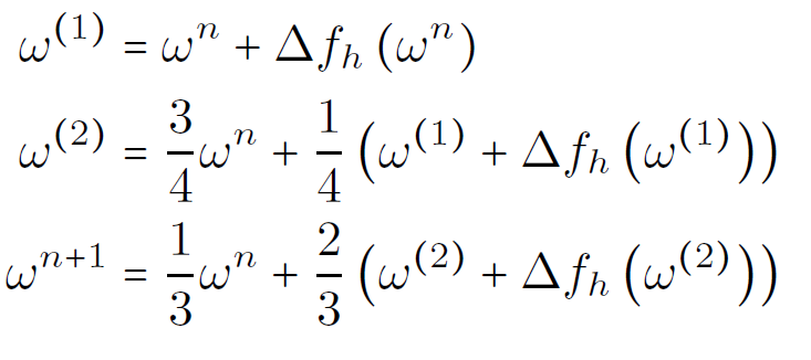
2D Euler equations: stochastic


Lie derivative
Sequence of indepentent Brownian motions

Filtered probability space
[Holm, 2015]
2D Euler equations: stochastic
eigenvectors of the velocity-velocity correlation tensor: divergence free
[Holm, 2015]


Transport velocity
Numerical scheme
-
SPACE: Galerkin finite elements
-
TIME: 3rd order Runge-Kutta
TIME: 3rd order Runge-Kutta


Combining SPACE-TIME


Consistency of the numerical method for the SPDE

Local truncation error

Local truncation error - deterministic

Def. For some γ>1, the discrete approximation operators S_Δ is called F-compatible if S_Δ is F_tj+1 measurable and
for all j=0,...,n-1.
Consistency of the numerical method for the SPDE
Def. We say that the numerical scheme S_Δ is consistent in mean square of order γ>1, w.r.t. the SPDE, if there exists a constant c independent on Δ ∈ (0,T], and for all ε>0 there exists 𝛿>0 such that for all 0<Δ<𝛿 and j=1,...,N:
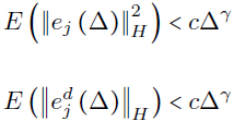
and S_Δ is F-compatible.
Consistency of the numerical method for the SPDE
Thm. Assuming the SPDE well-posed and for all T>0 and sufficiently large p, we have
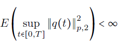
then the numerical schem S_Δ is consistent with γ=2.
[Crisan et al, 2018]
Calibration of the correlation eigenvectors
Assumptions in stochastic GFD


Averaged fluid particles equations of motion:
Eulerian stochastic QG equation
Estimation of the ξ
Deterministic unapproximated trajectories (fine grid):
Equations for ξ


Stochastic trajectories (coarse grid):
Methodology
- Spin up a fine grid simulation from t = −T_spin to t = 0 (till some statistical equilibrium is reached)
- Record velocity time series from t = 0 to t = MΔt
- Define as coarse grid points

For each m=0,...,M-1
- Solve for the initial data
and u(x,t) solution of the fine grid simulation


Methodology
- Compute by spatially averaging u over the coarse grid
- Compute by solving with the same initial condition
- Compute the difference
which measures the error between the fine and coarse trajectory


Finally, extract a basis for the noise minimizing:
N can be inferred by using EOFs

Numerical experiments for UQ
Initialization
- Solve deterministic PDE on a grid 512x512
- Coarse grain the solution to a grid 64x64 (thruth)
- spatial average of the stream function
- project it on the coarse grid
- The set of initial conditions at t0 is determined by letting the system to reach an energy equilibrium from an inital point at t_spin
- Time measured in ett = large eddy turnovers
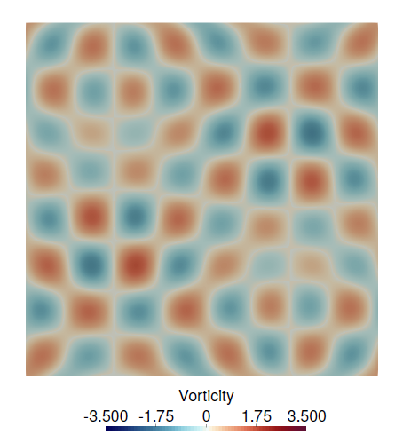
Initial vorticity at t_spin

Energy diagram
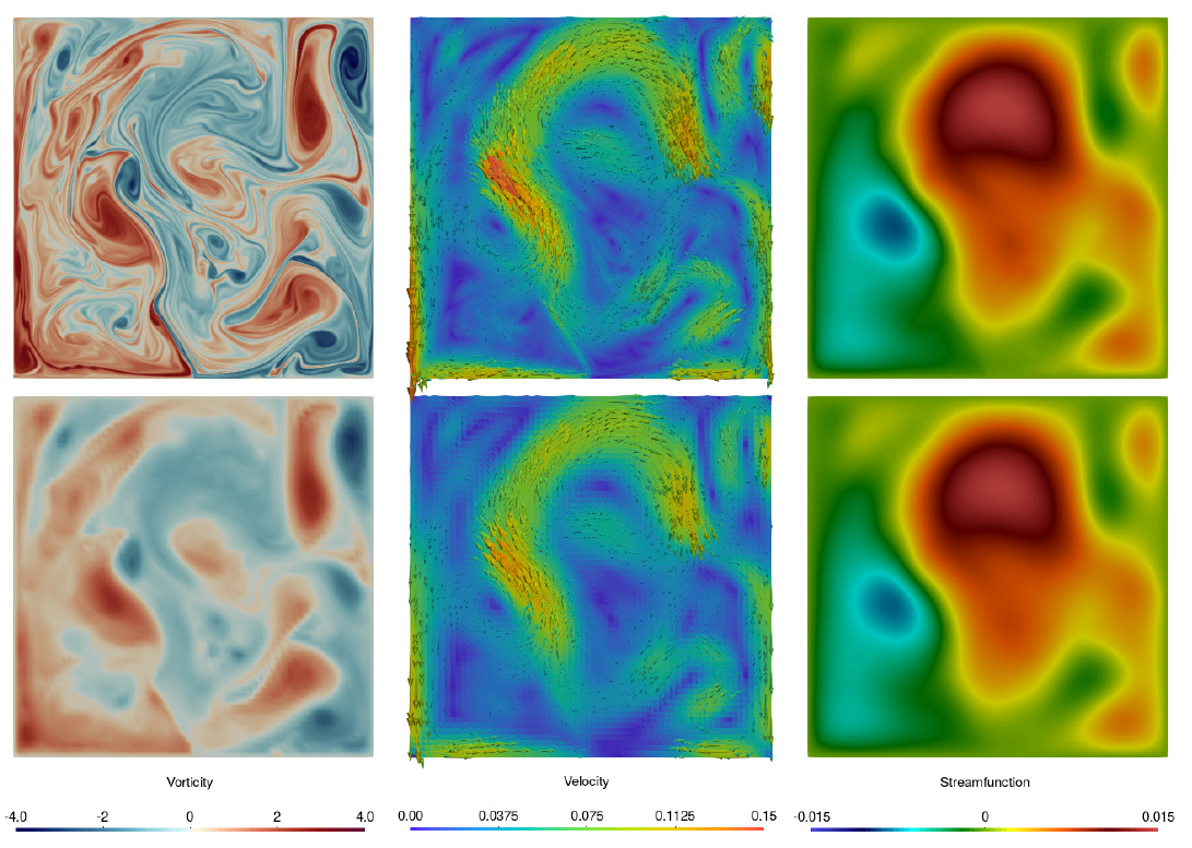
Vorticity
Velocity
Streamfunction
t = t0
Vorticity
Velocity
Streamfunction
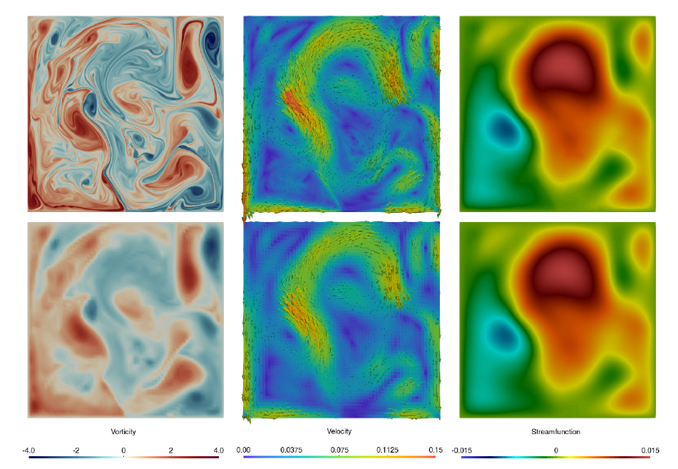
t = t0 + 146
Lagrangian trajectories and estimating the correlation eigenvectors
- Compute the difference
which measures the error between the fine and coarse trajectory
Finally, extract a basis for the noise minimizing:
N can be inferred by using EOFs


Uncertainty quantification test
- Substitute the computed ξ and simulate an ensemble of independent realisations of:
- Simulated 200 Lagrangian trajectories driven by the above equation, EOF capturing 90% of total variance
- Small time step: no significant deviations between the stochastic trajectories and the deterministic ones

SPDE ensemble and SPDE initial conditions
- SPDE run on a 64x64 grid
- An ensemble of Np initial conditions for the SPDE are
generated (each realization is called a particle)
- Goal when generating the initial conditions is to obtain an ensemble which contain particles that are "close"
to the truth.
- Done with a deformation process solving for 1-2 ett the SDE:

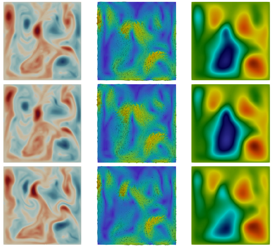
Vorticity
Velocity
Streamfunction
t = t0
Particle 1
Particle 2
Truth
Vorticity
Velocity
Streamfunction
t = t0 + 3
Particle 1
Particle 2
Truth
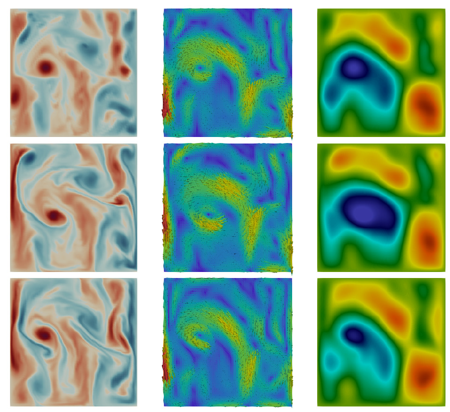
Vorticity
Velocity
Streamfunction
t = t0 + 5
Particle 1
Particle 2
Truth
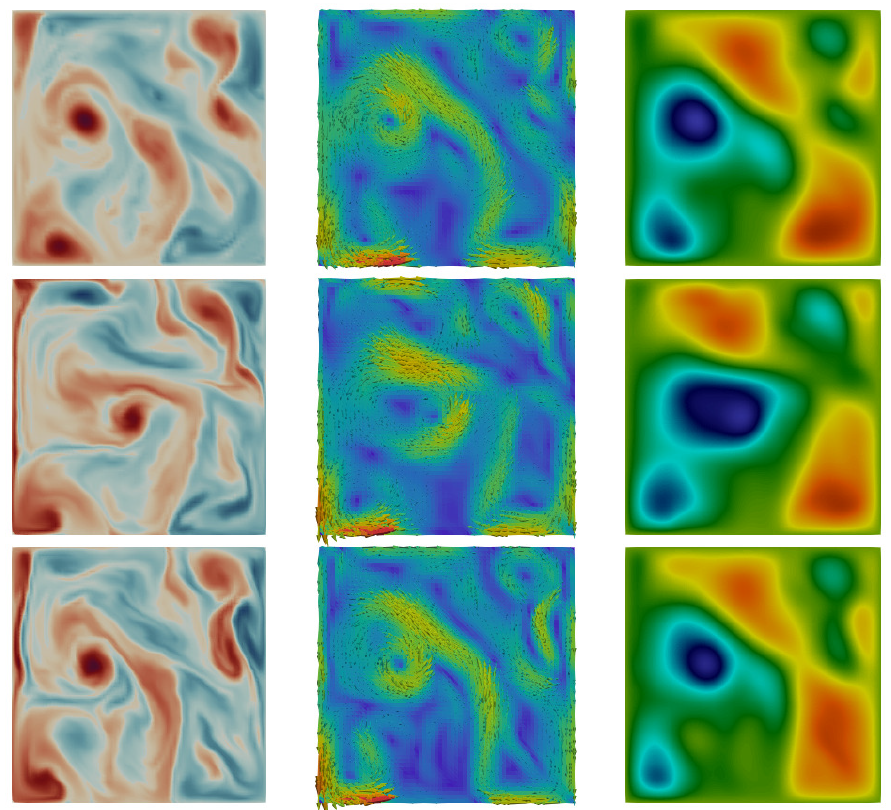
SPDE uncertainty quantification
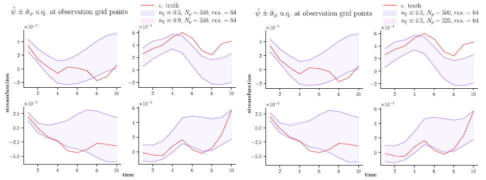
Uncertainty quanti cation plots comparing the truth with the ensemble one standard deviation region
about the ensemble mean for the streamfunction at four interior grid points of a 4 × 4 observation grid
Streamfunction
Uncertainty quanti cation plots comparing the truth with the ensemble one standard deviation region
about the ensemble mean for the streamfunction at four interior grid points of a 4 × 4 observation grid
Vorticity
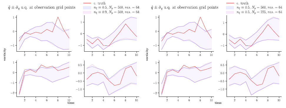
Uncertainty quanti cation plots comparing the truth with the ensemble one standard deviation region about the ensemble mean for the streamfunction at four interior grid points of a 4 × 4 observation grid
Streamfunction - different resolutions
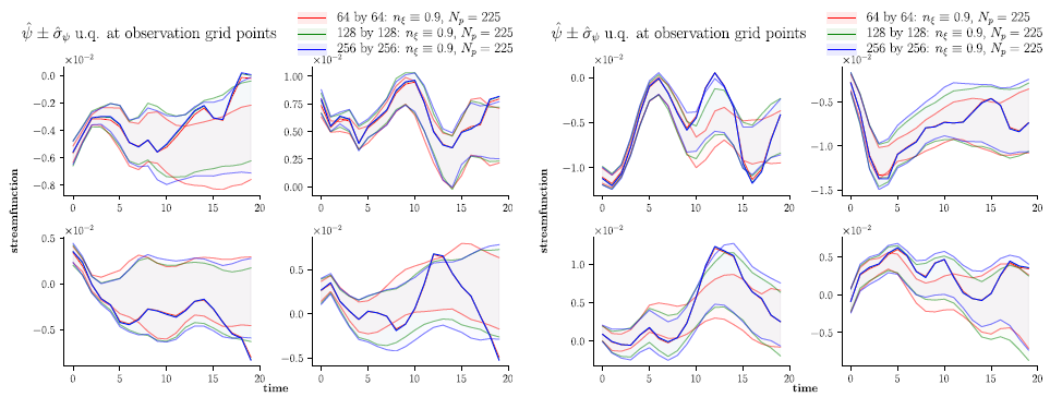
RMK: the coarse grid resolution gets re ned, the one
standard deviation region stays closer to the truth for longer time periods.
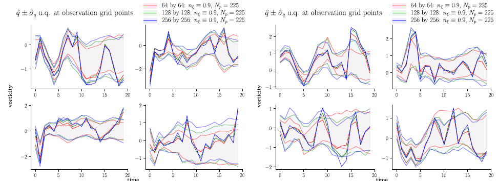
Uncertainty quanti cation plots comparing the truth with the ensemble one standard deviation region about the ensemble mean for the streamfunction at four interior grid points of a 4 × 4 observation grid
Vorticity - different resolutions
RMK: the coarse grid resolution gets re ned, the one
standard deviation region stays closer to the truth for longer time periods.
Conclusions
Conclusions
- New approach of data assimilation using the SALT equations: geometric mechanics-variational derivation
- Stable numerical method scheme for both stochastic and deterministic models
- UQ: the uncertainty decreases as the grid becomes more refined, and the fidelity to the true solution increases as the size of the ensemble increases
- Q: applying a geometric integrator would affect the UQ?