Milo Viviani 
(joint work with prof. Michele Benzi)

Scuola Normale Superiore - Pisa

Due Giorni di Algebra Lineare Numerica e Applicazioni
Napoli, 14-15 Febbraio 2022

Introduction

Isospectral flows

• \(Y_0\in \mathbb{M}(N,\mathbb{C})\), \(\mathcal{L}:\mathbb{M}(N,\mathbb{C})\rightarrow\mathbb{M}(N,\mathbb{C})\) linear
• \([A,B] = AB - BA\)
• The spectrum of \(Y\) is time-invariant
• \(\mathcal{L}\) self-adjoint w.r.t. Frobenious inner product \(\Rightarrow\) flow Hamiltonian w.r.t. \(H=\frac{1}{2}Tr(\mathcal{L}YY^*)\)

Geometric integration of isospectral flows

• Second order in time (\(h\) is the time-step)
• Spectrum of \(Y\) exactly preserved
• Hamiltonian conserved up to \(\mathcal{O}(h^2)\)

Cubic equation

• \(X\) unknown
• \(Y\in \mathbb{M}(N,\mathbb{R}) \ or \ \mathbb{M}(N,\mathbb{C})\) given

Thm. Given \(Y\in\mathbb{M}(N,\mathbb{C})\), equation (*) has a unique solution for sufficiently small \(h>0\) in some neighbourhood of \(Y\).
Furthermore, when equation (*) takes place in \(\mathfrak{su}(N)\), there exists such a neighbourhood for any \(h\leq\frac{1}{3\|\mathcal{L}\|_{op}\|Y\|}\).

Numerical schemes

Explicit fixed point iteration

• Convergence is guaranteed by the Theorem above, for  \(h\) sufficiently small and \(X_0:=Y\)
• The complexity is \(\mathcal{O}(N^3)\)
• Only two matrices multiplications are required when working in \(\mathfrak{su}(N)\)

Linear iteration

• Convergence can be derived by the Theorem above, for  \(h\) sufficiently small and \(X_0:=Y\)
• The complexity is \(\mathcal{O}(N^3)\)
• To solve the second equation we take the LU-factorization of \(I\pm hP_k\)

Inexact Newton iteration

\(G(X):=X - h[\mathcal{L} X,X]- h^2(\mathcal{L} X)X(\mathcal{L} X) - Y\)

\(DG(X)=I - h(\mathcal{B}_1 + h\mathcal{B}_2)\)

\(\mathcal{B}_2=(\mathcal{L}\cdot)X(\mathcal{L}X)+(\mathcal{L}X)\cdot(\mathcal{L}X)+(\mathcal{L}X)X(\mathcal{L}\cdot)\)

\(\mathcal{B}_1=[\mathcal{L}\cdot,X]+[\mathcal{L}X,\cdot]\)

Inexact Newton iteration

Need an approximation for \(DG(X)^{-1}\)

• \(DG(X)^{-1}\approx I + h\mathcal{B}_1\) [Exact 1st order]
• \(DG(X)^{-1}\approx I + h\mathcal{B}_1 + h^2\mathcal{B}_2\)
• \(DG(X)^{-1}\approx I + h\mathcal{B}_1 + h^2\mathcal{B}_1^2\)
• \(DG(X)^{-1}\approx I + h\mathcal{B}_1 + h^2(\mathcal{B}_1^2+\mathcal{B}_2)\) [Exact 2nd order]

Rmk. the second one is the best compromise between exactness and computational cost

• The total complexity is \(\mathcal{O}(N^3)\)

Numerical experiments

Euler Equations

Spatial semidiscretization of the Euler equations on a compact orientable surface \(S\), \(\omega_t\in C^\infty(S)\)

\(\dot{\omega}=\nabla\omega\cdot\nabla^\perp\Delta^{-1}\omega\)

Give the Hamiltonian isospectral flow on \(\mathfrak{su}(N)\), for \(N\geq 1\)

\(\dot{W}=[W,\Delta_N^{-1}W]\)

Rmk. \(\Delta_N\) is tridiagonal, the evaluation of \(\Delta_N^{-1}W\) (via LU-factorization done once) requires \(\mathcal{O}(N^2)\) operations

Euler Equations

Time-step \(h=0.5\), normalized initial data

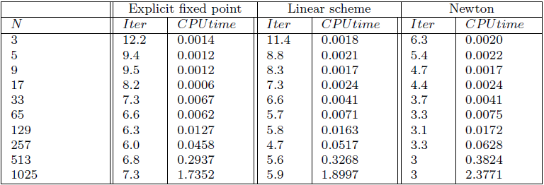
Rmk. Explicit fixed point performs the best in terms of CPU time

Heisenberg spin chain

Spatial semidiscretization of the Landau–Lifshitz–Gilbert Hamiltonian PDE, \(\sigma_t:S^1\rightarrow S^2\)

\(\dot{\sigma}=\sigma\times\partial_{xx}\sigma\)

Give the Hamiltonian isospectral flow on \(\mathfrak{su}(2)^{\oplus_N}\), for \(N\geq 1\)

\(\dot{S}_i=[S_i,S_{i-1}+S_{i+1}]\)

for \(i=1,...,N\) with \(S_1\equiv S_N\)

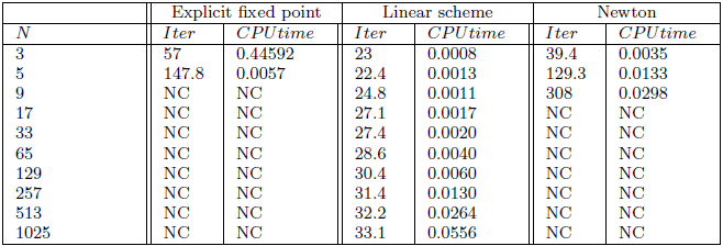
Time-step \(h=0.5\), normalized initial data

Rmk. Explicit fixed point performs the best in terms of stabilty and CPU time. 

Heisenberg spin chain

An unpractical scheme

Quadratic iteration

• The first equation is CARE (Continuous Algebraic Riccati Equation) in \(P_k\)
  
  
   
• Non-uniqueness issues

Conclusions

Conclusions

• Iterative schemes for the solution of cubic matrix equations arising in the numerical solution of certain conservative PDEs
• Geometrical integrators: preservation of important physical features
• Both fixed point iterations and inexact Newton work well
• Fixed point iterations more efficient for large time-step and large dimensions
• Implicit fixed point iteration is more stable

Thanks for your attention